Freiling G., Yurko V. Lectures on Differential Equations of Mathematical Physics: A First Course

Подождите немного. Документ загружается.

62 G.

Freiling and V. Yurko

4πt

f (x

−

−ρ

)

cos(n,x

)

Let f be

independent

of x

. Since cos( ¯n, ¯x

) =

−ρ

(see

ﬁg.

2.5.3), we have

w(x

) =

2π

σ(x

)

f (x

)

−ρ

)

−ρ

Figure

2.5.3.

particular, this yields that the function w(x

) does not depend on x

. Thus, if in

(2.5.1)-(2.5.2) the initial data ϕ and ψ do not depend on x

, then the solution also does

not depend on x

, and Kirchhoff’s formula (2.5.8) takes the form

u(x

) =

2π

∂

∂t

σ(x

)

ϕ(x

)

−ρ

2π

σ(x

)

ψ(x

)

−ρ

. (2.5.21)

Formula (2.5.21) is called the Poisson formula. It represents the solution of the Cauchy

problem (2.5.19)-(2.5.20).

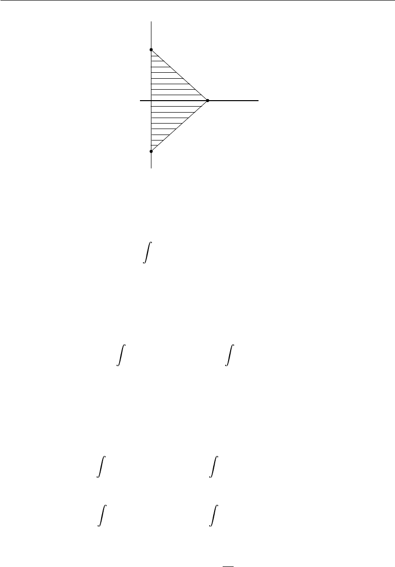
2) Let us make one more step in Hadamard’s method of descent. Suppose that in

(2.5.21) the functions ϕ and ψ do not depend on x

. Then

J :=

2π

σ(x

)

ϕ(x

)

−ρ

2π

−t

ϕ(x

−h

−ρ

where h

= t

−(x

−x

)

(see

ﬁg.

2.5.4).

Hyperbolic P

artial Differential Equations 63

−t

Figure

2.5.4.

Since

−h

−ρ

= arcsin

−x

−h

−

= π,

J =

−t

ϕ(x

Analogously

one transforms the second integral in (2.5.21). Thus, (2.5.21) takes the form

u(x

) =

ϕ(x

)

+ ϕ

−t

)

−t

ψ(x

. (

2.5.22)

Formula (2.5.22) is the D’Alembert formula (see Section 2.1), which gives the solution of

the Cauchy problem for the equation of a vibrating string:

= u

, −∞ < x < ∞, t > 0,

|t=0

= ϕ(x), u

t|t=0

= ψ(x).

)

(2.5.23)

Remark 2.5.1. The wave equations for n = 3, n = 2 and n = 1 are called the equations

of spherical, cylindrical and plane waves, respectively. The formulae (2.5.8), (2.5.21) and

(2.5.22) give us an opportunity to study the physical picture of wave propagation. We note

that for n = 3, the solution u(x

) depends on the initial data given only on the boundary

of the characteristic cone (i.e. on the sphere ∂K(x

) ). For n = 2 and n = 1, the solution

u(x

) depends on the initial data given on the whole base of the characteristic cone

(i.e. the circle σ(x

) or the segment [x

−t

+ t

] ). In other words, for n = 3

initial perturbations localized in the space produce in each point x

perturbations localized

with respect to time (Huygens’s principle), i.e. the wave has front and back wave fronts

(leading edge and trailing edge). For n = 2, initial perturbations localized in the space are

not localized with respect to time (the Huygens principle is not valid), i.e. the wave has a

leading edge and has no trailing edge - the oscillations will continue for inﬁnitely long time.

We note that the problem for n = 2 can be considered as a three-dimensional problem with

initial data given in an inﬁnite cylinder which do not depend on the third coordinate.

64 G.

Freiling and V. Yurko

2.6. An

Inverse Problem for the Wave Equation

Sections 2.6-2.9 contain a material for advanced studies, and they can be omitted ”in the

ﬁrst reading”. These sections are devoted to studying inverse problems for differential

equations. The Inverse problems that we study below consist in recovering coefﬁcients

of differential equations from characteristics which can be measured. Such problems often

appear in various areas of natural sciences and engineering (see [15]-[22] and the references

therein).

In this section we consider an inverse problem for a wave equation with a focused

source of disturbance. In applied problems the data are often functions of compact support

localized within a relative small area of space. It is convenient to model such situations

mathematically as problems with a focused source of disturbance.

Consider the following boundary value problem B(q(x),h) :

= u

−q(x)u, 0 ≤ x ≤t, (2.6.1)

u(x,x) = 1, (u

−hu)

|x=0,

(2.6.2)

where q(x) is a complex-valued locally integrable function (i.e. it is integrable on every

ﬁnite interval), and h is a complex number. Denote r(t) := u(0,t). The function r is

called the trace of the solution. In this section we study the following inverse problem.

Inverse Problem 2.6.1. Given the trace r(t), t ≥ 0, of the solution of B(q(x),h),

construct q(x), x ≥0, and h.

We prove an uniqueness theorem for Inverse Problem 2.6.1 (Theorem 2.6.3), provide

an algorithm for the solution of this inverse problem (Algorithm 2.6.1) and give necessary

and sufﬁcient conditions for its solvability (Theorem 2.6.4).

Remark 2.6.1. Let us note here that the boundary value problem B(q(x), h) is equiv-

alent to a Cauchy problem with a focused source of disturbance. For simplicity, we assume

here that h = 0. We deﬁne u(x,t) = 0 for 0 < t < x, and u(x,t) = u(−x,t), q(x) = q(−x)

for x < 0. Then, using symmetry, it follows that u(x,t) is a solution of the Goursat problem

= u

−q(x)u, 0 ≤ |x| ≤t,

u(x,|x|) = 1.

Moreover, it can be shown that this Goursat problem is equivalent to the Cauchy problem

= u

−q(x)u, −∞ < x < ∞, t > 0,

|t=0

= 0, u

t|t=0

= 2δ(x),

where δ(x) is the Dirac delta-function. Similarly, for h 6= 0, the boundary value problem

(2.6.1)-(2.6.2) also corresponds to a problem with a focused source of disturbance.

Let us return to the boundary value problem (2.6.1)-(2.6.2). Denote

Q(x) =

|q(t)|dt, Q

∗

(x) =

Q(t) dt, d = max(0,−h).

Hyperbolic P

artial Differential Equations 65

Theorem

2.6.1. The boundary value problem (2.6.1) −(2.6.2) has a unique solution

u(x,t), and

|u(x,t)| ≤ exp(d(t −x))exp

∗

t + x

¶¶

, 0 ≤x ≤t. (2.6.3)

oof

. We transform (2.6.1)-(2.6.2) by means of the replacement

ξ = t + x, η = t −x, v(ξ,η) = u

ξ −η

ξ + η

the

boundary value problem

ξη

(ξ,η) = −

ξ −η

v(ξ,η), 0 ≤ η ≤ξ, (2.6.4)

v(ξ,0)

= 1

, (v

(ξ,η) −v

(ξ,η) −hv(ξ,η))

|ξ=η

= 0. (2.6.5)

Since v

(ξ,0) = 0, integration of (2.6.4) with respect to η gives

(ξ,η) = −

ξ −α

v(ξ,α)dα. (2.6.6)

particular

, we have

(ξ,η)

|ξ=η

= −

η −α

v(η,α)dα. (2.6.7)

follo

ws from (2.6.6) that

v(ξ,η) = v(η,η) −

β −α

v(β,α)dα

dβ. (2.6.8)

Let

calculate v(η,η). Since

dη

(v(η,η)e

xp(

hη)) = (v

(ξ,η) + v

(ξ,η) + hv(ξ,η))

|ξ=η

exp(hη),

we get by virtue of (2.6.5) and (2.6.7),

dη

(v(η,η)e

xp(h

η)) = 2v

(ξ,η)

|ξ=η

exp(hη)

= −

xp(h

η)

η −α

v(η,α)dα.

This

yields

(with v(0,0) = 1 )

v(η,η)exp(hη)−1 = −

xp(h

β)

β −α

v(β,α)dα

dβ,

66 G.

Freiling and V. Yurko

and consequently

v(η,η)

= exp(−hη)

−

xp(−h

(η −β))

β −α

v(β,α)dα

dβ. (2.6.9)

Substituting

(2.6.9)

into (2.6.8) we deduce that the function v(ξ,η) satisﬁes the integral

equation

v(ξ,η) = exp(−hη)

−

xp(−h

(η −β))

β −α

v(β,α)dα

dβ

−

β −α

v(β,α)dα

dβ. (2.6.10)

Con

ersely, if v(ξ,η) is a solution of (2.6.10) then one can verify that v(ξ,η) satisﬁes

(2.6.4)-(2.6.5).

We solve the integral equation (2.6.10) by the method of successive approximations.

The calculations are slightly different for h ≥ 0 and h < 0.

Case 1. Let h ≥ 0. Denote

(ξ,η) = exp(−hη),

k+1

(ξ,η) = −

xp(−h

(η −β))

β −α

(β,α)dα

dβ

−

β −α

(β,α)dα

dβ. (2.6.11)

Let

show by induction that

(ξ,η)| ≤

∗

¶¶

, k ≥ 0, 0 ≤η ≤ ξ. (2.6.12)

Indeed,

for k = 0

, (2.6.12) is obvious. Suppose that (2.6.12) is valid for a certain k ≥0.

It follows from (2.6.11) that

k+1

(ξ,η)| ≤

β −α

(β,α)

dα

dβ. (2.6.13)

Substituting

(2.6.12)

into the right-hand side of (2.6.13) we obtain

k+1

(ξ,η)| ≤

2k!

∗

¶¶

β −α

dα

dβ

≤

∗

¶¶

β/2

|q(s)|d

dβ

∗

¶¶

dβ

Hyperbolic P

artial Differential Equations 67

ξ/2

(2Q

∗

(s))

(2Q

∗

(s))

s =

(k + 1)!

∗

¶¶

k+1

;

hence

(2.6.12)

is valid.

It follows from (2.6.12) that the series

v(ξ,η) =

∞

∑

k=0

(ξ,η)

converges absolutely and uniformly on compact sets 0 ≤η ≤ξ ≤ T, and

|v(ξ,η)| ≤ exp

∗

¶¶

The

function v

(ξ,η) is the unique solution of the integral equation (2.6.10). Consequently,

the function u(x,t) = v(t + x,t −x) is the unique solution of the boundary value problem

(2.6.1)-(2.6.2), and (2.6.3) holds.

Case 2. Let h < 0. we transform (2.6.10) by means of the replacement

w(ξ,η) = v(ξ,η) exp(hη)

to the integral equation

w(ξ,η) = 1 −

β −α

xp(h

(β −α))w(β,α)dα

dβ

−

β −α

xp(h

(η −α))w(β,α)dα

dβ. (2.6.14)

By the method of successive approximations we get similarly to Case 1 that the integral

equation (2.6.14) has a unique solution, and that

|w(ξ,η)| ≤ exp

∗

¶¶

i.e.

Theorem

2.6.1 is proved also for h < 0. 2

Remark 2.6.2. It follows from the proof of Theorem 2.6.1 that the solution u(x,t)

of (2.6.1)-(2.6.2) in the domain Θ

:= {(x,t) : 0 ≤ x ≤ t, 0 ≤ x + t ≤ 2T } is uniquely

determined by the speciﬁcation of h and q(x) for 0 ≤x ≤T, i.e. if q(x) = ˜q(x), x ∈[0, T ]

and h =

h, then u(x,t) = ˜u(x,t) for (x,t) ∈ Θ

. Therefore, one can also consider the

boundary value problem (2.6.1)-(2.6.2) in the domains Θ

and study the inverse problem

of recovering q(x), 0 ≤ x ≤T and h from the given trace r(t), t ∈ [0,2T ].

Denote by D

(N ≥0) the set of functions f (x), x ≥0 such that for each ﬁxed T > 0,

the functions f

( j)

(x), j =

0,N −1 are

absolutely

continuous on [0, T ], i.e. f

( j)

(x) ∈

L(0,T ), j =

0,N. It

follo

ws from the proof of Theorem 2.6.1 that r(t) ∈ D

, r(0) =

1, r

(0) = −h. Moreover, the function r

has the same smoothness properties as the po-

tential q. For example, if q ∈D

then r ∈ D

N+2

68 G.

Freiling and V. Yurko

In order

to solve Inverse Problem 2.6.1 we will use the Riemann formula for the solution

of the Cauchy problem

−p(t)u = u

−q(x)u + p

(x,t),

−∞ < x < ∞, t > 0,

|t=0

= r(x), u

t|t=0

= s(x).











(2.6.15)

According to the Riemann formula (see Section 2.4) the solution of (2.6.15) has the form

u(x,t) =

(r(x +t)

+ r(x −t))

x+t

x−t

(s(ξ)R(ξ,0,x,t) −r(ξ)R

(ξ,0,x,t)) dξ

dτ

x+t−τ

x+τ−t

R(ξ,τ,x,t)p

(ξ,τ)dξ,

where R(ξ,τ, x,t) is

the

Riemann function, and R

∂R

∂τ

. Note

that

if q(x) ≡ const, then

R(ξ,τ,x,t) = R(ξ −x,τ,t). In particular, the solution of the Cauchy problem

= u

−q(x)u, −∞ < t < ∞, x > 0,

|x=0

= r(t), u

x|x=0

= hr(t),

)

(2.6.16)

has the form

u(x,t) =

(r(t + x)

+ r(t −x))

−

t+x

t−x

r(ξ)(R

(ξ −t,0, x) −hR(ξ −t,0,x))dξ.

The

change

of variables τ = t −ξ leads to

u(x,t) =

(r(t + x)

+ r(t −x))

−x

r(t −τ)G(x, τ)dτ, (2.6.17)

where G(x,τ)

= −R

(

−τ,0,x) + hR(−τ,0,x).

Let us take r(t) = cos ρt in (2.6.16), and let ϕ(x, λ) be the solution of the equation

−ϕ

(x,λ) + q(x)ϕ(x,λ) = λϕ(x,λ), λ = ρ

under the initial conditions ϕ(0,λ) = 1, ϕ

(0,λ) = h. Obviously, the function u(x,t) =

ϕ(x,λ) cosρt is a solution of problem (2.6.16). Therefore, (2.6.17) yields for t = 0,

ϕ(x,λ) = cos ρx +

−x

G(x,τ) cosρτ dτ.

Since G(x,−τ)

= G(x,τ

), we have

ϕ(x,λ) = cos ρx +

G(x,τ) cosρτ dτ.

Hyperbolic P

artial Differential Equations 69

Hence

(x,λ) = −ρsinρ

x + G(x,x)cosρx +

(x,τ) cosρτ dτ,

G(0,0) = h,

(x,λ) = −ρ

cosρx −G(x,x)ρsin ρx +

dG(x,x)

cosρ

(x,t)

|t=x

cosρx +

(x,τ) cosρτ dτ,

λϕ(x,λ) = ρ

cosρx + ρ

G(x,τ) cosρτ dτ.

Integration by parts yields

λϕ(x,λ) = ρ

cosρx + G(x,x)ρsin ρx + G

(x,t)

|t=x

cosρx

−G

(x,t)

|t=0

−

(x,τ) cosρτ dτ.

Since ϕ

(x,λ) + λϕ(x,λ) −q(x)ϕ(x,λ) = 0 and

(x,t) + G

(x,t))

|t=x

dG(x,x)

follows that

dG(x,x)

−q

(x)

cosρx −G

(x,t)

|t=0

(x,τ) −G

(x,τ) −q(x)G(x,τ)

cosρτ dτ = 0,

and consequently,

dG(x,x)

= q

(x), G

(x,t)

|t=0

= 0,

(x,τ) = G

(x,τ) −q(x)G(x,τ).

Thus, we have proved that

q(x) = 2

dG(x,x)

, G(0

,0) = h,

hence

G(x,x) = h +

q(t) d

t. (

2.6.18)

Let us go on to the solution of Inverse Problem 2.6.1. Let u(x,t) be the solution of

the boundary value problem (2.6.1)-(2.6.2). We deﬁne u(x,t) = 0 for 0 ≤ t < x, and

u(x,t) = −u(x,−t), r(t) = −r(−t) for t < 0. Then u(x,t) is the solution of the Cauchy

problem (2.6.16), and consequently (2.6.17) holds. But u(x,t) = 0 for x > |t| (this is a

connection between q(x) and r(t) ), and hence

(r(t + x)

+ r(t −x)

) +

−x

r(t −τ)G(x, τ)dτ = 0, |t| < x. (2.6.19)

70 G.

Freiling and V. Yurko

Denote a(t) = r

(t). Dif

ferentiating (2.6.19) with respect to t and using the relations

r(0+) = 1, r(0−) = −1, (2.6.20)

we obtain

G(x,t) + F(x,t) +

G(x,τ)F(t, τ)dτ = 0, 0 < t < x, (2.6.21)

where

F(x,t) =

(a(t + x)

+ a

(t −x)) (2.6.22)

with a(t) = r

(t). Equation (2.6.21) is called the Gelfand-Levitan equation for the Inverse

Problem 2.6.1.

Theorem 2.6.2. For each ﬁxed x > 0, equation (2.6.21) has a unique solution.

Proof. Fix x

> 0. It is sufﬁcient to prove that the homogeneous equation

g(t) +

g(τ)F(t,τ)dτ = 0, 0 ≤t ≤x

(2.6.23)

has only the trivial solution g(t) = 0.

Let g(t), 0 ≤t ≤ x

be a solution of (2.6.23). Since a(t) = r

(t) ∈ D

, it follows from

(2.6.22) and (2.6.23) that g(t) is an absolutely continuous function on [0,x

]. We deﬁne

g(−t) = g(t) for t ∈ [0,x

], and furthermore g(t) = 0 for |t| > x

Let us show that

−x

r(t −τ)g(τ)dτ = 0, t ∈ [−x

]. (2.6.24)

Indeed, by virtue of (2.6.20) and (2.6.23), we have

−x

r(t −τ

)g(τ)dτ

−x

r(t −τ

)g(τ)dτ +

r(t −τ)g(τ)dτ

= r(+0)g(t) −r(−0)g(t) +

−x

a(t −τ)g(τ)dτ

= 2

g(t) +

g(τ)F(t,τ)dτ

= 0.

Consequently,

−x

r(t −τ)g(τ)dτ ≡C

Taking here t = 0 and using that r(−τ)g(τ) is an odd function, we calculate C

= 0, i.e.

(2.6.24) is valid.

Hyperbolic P

artial Differential Equations 71

∆

−x

Figure

2.6.1.

Denote ∆

= {

(x,t) : x −x

≤t ≤ x

−x, 0 ≤ x ≤x

} and consider the function

w(x,t) :=

∞

−∞

u(x,t −τ)g(τ) dτ, (x,t) ∈ ∆

, (2.6.25)

where u(x,t) is the solution of the boundary value problem (2.6.1)-(2.6.2). Let us show

that

w(x,t) = 0, (x,t) ∈ ∆

. (2.6.26)

Since u(x,t) = 0 for x > |t|, (2.6.25) takes the form

w(x,t) =

t−x

−∞

u(x,t −τ)g(τ) dτ +

∞

t+x

u(x,t −τ)g(τ) dτ. (2.6.27)

Differentiating (2.6.27) and using the relations

u(x,x) = 1, u(x,−x) = −1, (2.6.28)

we calculate

(x,t) = g(t + x) −g(t −x)

t−x

−∞

(x,t −τ)g(τ) dτ +

∞

t+x

(x,t −τ)g(τ) dτ, (2.6.29)

(x,t) = g(t + x) + g(t −x)

t−x

−∞

(x,t −τ)g(τ) dτ +

∞

t+x

(x,t −τ)g(τ) dτ. (2.6.30)

Since, in view of (2.6.28),

(x,t) ±u

(x,t)

|t=±x

(x,±x) = 0,

it follows from (2.6.29)-(2.6.30) that

(x,t) −w

(x,t) −q(x)w(x,t)