Greene W.H. Econometric Analysis
Подождите немного. Документ загружается.


CHAPTER 21
✦
Nonstationary Data
949
TABLE 21.2
Critical Values for the Dickey–Fuller DF
τ
Test
Sample Size
25 50 100 ∞
F ratio (D–F)
a
7.24 6.73 6.49 6.25
F ratio (standard) 3.42 3.20 3.10 3.00
AR model
b
(random walk)
0.01 −2.66 −2.62 −2.60 −2.58
0.025 −2.26 −2.25 −2.24 −2.23
0.05 −1.95 −1.95 −1.95 −1.95
0.10 −1.60 −1.61 −1.61 −1.62
0.975 1.70 1.66 1.64 1.62
AR model with constant (random walk with drift)
0.01 −3.75 −3.59 −3.50 −3.42
0.025 −3.33 −3.23 −3.17 −3.12
0.05 −2.99 −2.93 −2.90 −2.86
0.10 −2.64 −2.60 −2.58 −2.57
0.975 0.34 0.29 0.26 0.23
AR model with constant and time trend (trend stationary)
0.01 −4.38 −4.15 −4.04 −3.96
0.025 −3.95 −3.80 −3.69 −3.66
0.05 −3.60 −3.50 −
3.45 −3.41
0.10 −3.24 −3.18 −3.15 −3.13
0.975 −0.50 −0.58 −0.62 −0.66
a
From Dickey and Fuller (1981, p. 1063). Degrees of freedom are 2 and T − p −3.
b
From Fuller (1976, p. 373 and 1996, Table 10.A.2).
with the revised set of critical values may be used for a one-sided test. Critical values for
this test are shown in the top panel of Table 21.2. Note that in general, the critical value
is considerably larger in absolute value than its counterpart from the t distribution. The
second approach is based on the statistic
DF
γ
= T( ˆγ − 1).
Critical values for this test are shown in the top panel of Table 21.2.
The simple random walk model is inadequate for many series. Consider the rate
of inflation from 1950.2 to 2000.4 (plotted in Figure 21.4) and the log of GDP over the
same period (plotted in Figure 21.5). The first of these may be a random walk, but it
is clearly drifting. The log GDP series, in contrast, has a strong trend. For the first of
these, a random walk with drift may be specified,
y
t
= μ + z
t
,
z
t
= γ z
t−1
+ ε
t
,
or
y
t
= μ(1 − γ)+ γ y
t−1
+ ε
t
.
For the second type of series, we may specify the trend stationary form,
y
t
= μ + βt + z
t
,
z
t
= γ z
t−1
+ ε
t

950
PART V
✦
Time Series and Macroeconometrics
1950
5
20
15
10
5
0
Quarter
Chg.CPIU
1963 1976 20021989
Rate of Inflation, 1950.2 to 2000.4
FIGURE 21.4
Rate of Inflation in the Consumer Price Index.
1950
7.25
7.50
Quarter
LogGDP
Log of GDP, 1950.1 to 2000.4
1963 1976 20021989
7.75
8.00
8.25
8.50
8.75
9.00
9.25
FIGURE 21.5
Log of Gross Domestic Product.
or
y
t
= [μ(1 − γ)+ γβ] + β(1 − γ)+ γ y
t−1
+ ε
t
.
The tests for these forms may be carried out in the same fashion. For the model with
drift only, the center panels of Tables 21.2 and 21.3 are used. When the trend is included,
the lower panel of each table is used.

CHAPTER 21
✦
Nonstationary Data
951
TABLE 21.3
Critical Values for the Dickey–Fuller DF
γ
Test
Sample Size
25 50 100 ∞
AR model
a
(random walk)
0.01 −11.8 −12.8 −13.3 −13.8
0.025 −9.3 −9.9 −10.2 −10.5
0.05 −7.3 −7.7 −7.9 −8.1
0.10 −5.3 −5.5 −5.6 −5.7
0.975 1.78 1.69 1.65 1.60
AR model with constant (random walk with drift)
0.01 −17.2 −18.9 −19.8 −20.7
0.025 −14.6 −15.7 −16.3 −16.9
0.05 −12.5 −13.3 −13.7 −14.1
0.10 −10.2 −10.7 −11.0 −11.3
0.975 0.65 0.53 0.47 0.41
AR model with constant and time trend (trend stationary)
0.01 −22.5 −25.8 −27.4 −29.4
0.025 −20.0 −22.4 −23.7 −24.4
0.05 −17.9 −19.7 −
20.6 −21.7
0.10 −15.6 −16.8 −17.5 −18.3
0.975 −1.53 −1.667 −1.74 −1.81
a
From Fuller (1976, p. 373 and 1996, Table 10.A.1).
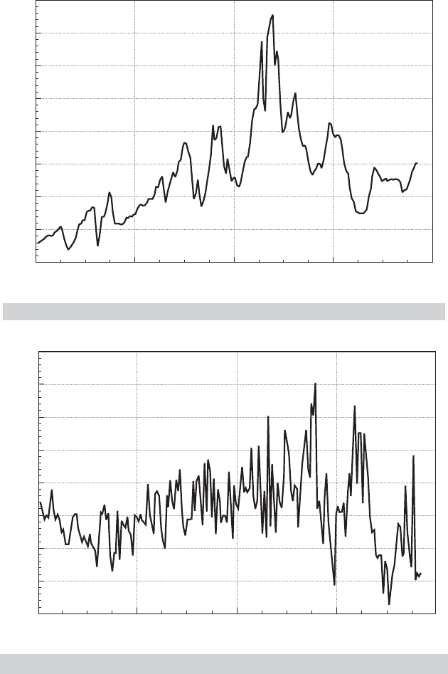
Example 21.2 Tests for Unit Roots
Cecchetti and Rich (2001) studied effect of recent monetary policy on the U.S. economy. The
data used in their study were the following variables:
π = one period rate of inflation = the rate of change in the CPI
y = log of real GDP
i = nominal interest rate = the quarterly average yield on a 90-day T-bill
m = change in the log of the money stock, M1
i − π = ex post real interest rate
m − π = real growth in the money stock
Data used in their analysis were from the period 1959.1 to 1997.4. As part of their analysis,
they checked each of these series for a unit root and suggested that the hypothesis of a unit
root could only be rejected for the last two variables. We will reexamine these data for the
longer interval, 1950.2 to 2000.4. The data are in Appendix Table F5.2. Figures 21.6 through
21.9 show the behavior of the last four variables. The first two are shown in Figures 21.4 and
21.5. Only the real output figure shows a strong trend, so we will use the random walk with
drift for all the variables except this one.
The Dickey–Fuller tests are carried out in Table 21.4. There are 203 observations used in
each one. The first observation is lost when computing the rate of inflation and the change
in the money stock, and one more is lost for the difference term in the regression. The
critical values from interpolating to the second row, last column in each panel for 95 percent
significance and a one-tailed test are −3.68 and −24.2, respectively, for DF
τ
and DF
γ
for the
output equation, which contains the time trend, and −3.14 and −16.8 for the other equations,
which contain a constant but no trend. For the output equation ( y) , the test statistics are
DF
τ
=
0.9584940384 − 1
.017880922
=−2.32 > −3.44,
952
PART V
✦
Time Series and Macroeconometrics
1950
0
2
Quarter
T-Bill Rate
1963 1976 20021989
4
6
8
10
12
14
16
FIGURE 21.6
T-Bill Rate.
6
5
4
3
2
1
0
1
2
M1
1950 1963 1976 1989
Quarter
2002
FIGURE 21.7
Change in the Money Stock.
and
DF
γ
= 202(0.9584940384 − 1) =−8.38 > −21.2.
Neither is less than the critical value, so we conclude (as have others) that there is a unit root
in the log GDP process. The results of the other tests are shown in Table 21.4. Surprisingly,
CHAPTER 21
✦
Nonstationary Data
953
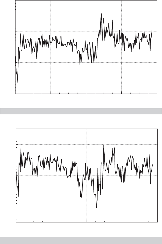
15
10
5
0
5
10
15
Real Interest Rate
1950 1963 1976 1989 2002
Quarter
FIGURE 21.8
Ex Post Real T-Bill Rate.
10
5
0
5
10
15
20
Real M1
1950 1963 1976 1989 2002
Quarter
FIGURE 21.9
Change in the Real Money Stock.
these results do differ sharply from those obtained by Cecchetti and Rich (2001) for π and
m. The sample period appears to matter; if we repeat the computation using Cecchetti
and Rich’s interval, 1959.4 to 1997.4, then DF
τ
equals −3.51. This is borderline, but less
contradictory. For m we obtain a value of −4.204 for DF
τ
when the sample is restricted to
the shorter interval.

954
PART V
✦
Time Series and Macroeconometrics
TABLE 21.4
Unit Root Tests (Standard errors of estimates in parentheses)
μβγDF
τ
DF
γ
Conclusion
π 0.332 0.659 −6.40 −68.88 Reject H
0
(0.0696) (0.0532) R
2
= 0.432, s = 0.643
y 0.320 0.00033 0.958 −2.35 −8.48 Do not reject H
0
(0.134) (0.00015) (0.0179) R
2
= 0.999, s = 0.001
i 0.228 0.961 −2.14 −7.88 Do not reject H
0
(0.109) (0.0182) R
2
= 0.933, s = 0.743
m 0.448 0.596 −7.05 −81.61 Reject H
0
(0.0923) (0.0573) R
2
= 0.351, s = 0.929
i − π 0.615 0.557 −7.57 −89.49 Reject H
0
(0.185) (0.0585) R
2
= 0.311, s = 2.395
m − π 0.0700 0.490 −8.25 −103.02 Reject H
0
(0.0833) (0.0618) R
2
= 0.239, s = 1.176
The Dickey–Fuller tests described in this section assume that the disturbances in the
model as stated are white noise. An extension which will accommodate some forms of
serial correlation is the augmented Dickey–Fuller test. The augmented Dickey–Fuller
test is the same one as described earlier, carried out in the context of the model
y
t
= μ + βt + γ y
t−1
+ γ
1
y
t−1
+···+γ
p
y
t−p
+ ε
t
.
The random walk form is obtained by imposing μ = 0 and β = 0; the random walk
with drift has β =0; and the trend stationary model leaves both parameters free. The
two test statistics are
DF
τ
=
ˆγ − 1
Est. Std. Error( ˆγ)
,
exactly as constructed before, and
DF
γ
=
T( ˆγ − 1)
1 − ˆγ
1
−···−ˆγ
p
.
The advantage of this formulation is that it can accommodate higher-order autoregres-
sive processes in ε
t
.
An alternative formulation may prove convenient. By subtracting y
t−1
from both
sides of the equation, we obtain
y
t
= μ + βt + γ
∗
y
t−1
+
p
j=1
φ
j
y
t−j
+ ε
t
,
where
φ
j
=−
p
k=j+1
γ
k
and γ
∗
=
p
i=1
γ
i
− 1.
The unit root test is carried out as before by testing the null hypothesis γ
∗
=0 against
γ
∗
< 0.
10
The t test, DF
τ
, may be used. If the failure to reject the unit root is taken as
10
It is easily verified that one of the roots of the characteristic polynomial is 1/(γ
1
+ γ
2
+···+γ
p
).

CHAPTER 21
✦
Nonstationary Data
955
evidence that a unit root is present, that is, γ
∗
=0, then the model specializes to the
AR(p − 1) model in the first differences which is an ARIMA(p −1, 1, 0) model for y
t
.
For a model with a time trend,
y
t
= μ + βt + γ
∗
y
t−1
+
p−1
j=1
φ
j
y
t−j
+ ε
t
,
the test is carried out by testing the joint hypothesis that β =γ
∗
=0. Dickey and Fuller
(1981) present counterparts to the critical F statistics for testing the hypothesis. Some of
their values are reproduced in the first row of Table 21.2. (Authors frequently focus on
γ
∗
and ignore the time trend, maintaining it only as part of the appropriate formulation.
In this case, one may use the simple test of γ
∗
=0 as before, with the DF
τ
critical values.)
The lag length, p, remains to be determined. As usual, we are well advised to
test down to the right value instead of up. One can take the familiar approach and
sequentially examine the t statistic on the last coefficient—the usual t test is appropriate.
An alternative is to combine a measure of model fit, such as the regression s
2
with one
of the information criteria. The Akaike and Schwarz (Bayesian) information criteria
would produce the two information measures
IC( p) = ln
e
e
T − p
max
− K
∗
+ ( p + K
∗
)
A
∗
T − p
max
− K
∗
,
K
∗
= 1 for random walk, 2 for random walk with drift, 3 for trend stationary,
A
∗
= 2 for Akaike criterion, ln(T − p
max
− K
∗
) for Bayesian criterion,
p
max
= the largest lag length being considered.
The remaining detail is to decide upon p
max
. The theory provides little guidance here.
On the basis of a large number of simulations, Schwert (1989) found that
p
max
= integer part of [12 × (T/100)
.25
]
gave good results.
Many alternatives to the Dickey–Fuller tests have been suggested, in some cases
to improve on the finite sample properties and in others to accommodate more general
modeling frameworks. The Phillips (1987) and Phillips and Perron (1988) statistic may
be computed for the same three functional forms,
y
t
= δ
t
+ γ y
t−1
+ γ
1
y
t−1
+···+γ
p
y
t−p
+ ε
t
, (21-6)
where δ
t
may be 0,μ,orμ +βt. The procedure modifies the two Dickey–Fuller statistics
we previously examined:
Z
τ
=
4
c
0
a
ˆγ − 1
v
−
1
2
(a − c
0
)
Tv
√
as
2
,
Z
γ
=
T( ˆγ − 1)
1 − ˆγ
1
−···−ˆγ
p
−
1
2
T
2
v
2
s
2
(a − c
0
),

956
PART V
✦
Time Series and Macroeconometrics
where
s
2
=
T
t=1
e
2
t
T − K
,
v
2
= estimated asymptotic variance of ˆγ,
c
j
=
1
T
T
s=j+1
e
t
e
t−s
, j = 0,...,L = jth autocovariance of residuals,
c
0
= [(T − K)/T]s
2
,
a = c
0
+ 2
L
j=1
1 −
j
L + 1
c
j
.
[Note the Newey–West (Bartlett) weights in the computation of a. As before, the analyst
must choose L.] The test statistics are referred to the same Dickey–Fuller tables we have
used before.
Elliot, Rothenberg, and Stock (1996) have proposed a method they denote the
ADF-GLS procedure, which is designed to accommodate more general formulations
of ε; the process generating ε
t
is assumed to be an I(0) stationary process, possibly an
ARMA(r, s). The null hypothesis, as before, is γ = 1 in (21-6) where δ
t
= μ or μ + βt.
The method proceeds as follows:
Step 1. Linearly regress
y
∗
=
⎡
⎢
⎣
y
1
y
2
− ¯ry
1
···
y
T
− ¯ry
T −1
⎤
⎥
⎦
on X
∗
=
⎡
⎢
⎣
1
1 − ¯r
···
1 − ¯r
⎤
⎥
⎦
or X
∗
=
⎡
⎢
⎣
11
1 − ¯r 2 − ¯r
···
1 − ¯rT− ¯r ( T − 1)
⎤
⎥
⎦
for the random walk with drift and trend stationary cases, respectively. (Note that the
second column of the matrix is simply ¯r + (1 − ¯r )t.) Compute the residuals from this
regression, ˜y
t
= y
t
−
ˆ
δ
t
.¯r = 1 −7/T for the random walk model and 1 −13.5/T for the
model with a trend.
Step 2. The Dickey–Fuller DF
τ
test can now be carried out using the model
˜y
t
= γ ˜y
t−1
+ γ
1
˜y
t−1
+···+γ
p
˜y
t−p
+ η
t
.
If the model does not contain the time trend, then the t statistic for (γ − 1) may be
referred to the critical values in the center panel of Table 21.2. For the trend stationary
model, the critical values are given in a table presented in Elliot et al. The 97.5 percent
critical values for a one-tailed test from their table is −3.15.
As in many such cases of a new technique, as researchers develop large and small
modifications of these tests, the practitioner is likely to have some difficulty deciding how
to proceed. The Dickey–Fuller procedures have stood the test of time as robust tools

CHAPTER 21
✦
Nonstationary Data
957
that appear to give good results over a wide range of applications. The Phillips–Perron
tests are very general but appear to have less than optimal small sample properties.
Researchers continue to examine it and the others such as Elliot et al. method. Other
tests are catalogued in Maddala and Kim (1998).
Example 21.3 Augmented Dickey–Fuller Test for a Unit Root in GDP
The Dickey–Fuller 1981 JASA paper is a classic in the econometrics literature—it is probably
the single most frequently cited paper in the field. It seems appropriate, therefore, to revisit at
least some of their work. Dickey and Fuller apply their methodology to a model for the log of
a quarterly series on output, the Federal Reserve Board Production Index. The model used is
y
t
= μ + βt + γ y
t−1
+ φ( y
t−1
− y
t−2
) + ε
t
. (21-7)
The test is carried out by testing the joint hypothesis that both β and γ
∗
are zero in the model
y
t
− y
t−1
= μ
∗
+ βt + γ
∗
y
t−1
+ φ( y
t−1
− y
t−2
) + ε
t
.
(If γ =0, then μ
∗
will also by construction.) We will repeat the study with our data on real GDP
from Appendix Table F5.2 using observations 1950.1 to 2000.4.
We will use the augmented Dickey–Fuller test first. Thus, the first step is to determine
the appropriate lag length for the augmented regression. Using Schwert’s suggestion, we
find that the maximum lag length should be allowed to reach p
max
={the integer part of
12[204/100]
.25
}=14. The specification search uses observations 18 to 204, because as many
as 17 coefficients will be estimated in the equation
y
t
= μ + βt + γ y
t−1
+
p
j =1
γ
j
y
t−j
+ ε
t
.
In the sequence of 14 regressions with j = 14, 13, ..., the only statistically significant lagged
difference is the first one, in the last regression, so it would appear that the model used by
Dickey and Fuller would be chosen on this basis. The two information criteria produce a similar
conclusion. Both of them decline monotonically from j =14 all the way down to j =1, so on
this basis, we end the search with j =1, and proceed to analyze Dickey and Fuller’s model.
The linear regression results for the equation in (21-7) are
y
t
= 0.368 + 0.000391t + 0.952y
t−1
+ 0.36025y
t−1
+ e
t
, s = 0.00912
(0.125) (0.000138) (0.0167) (0.0647) R
2
= 0.999647.
The two test statistics are
DF
τ
=
0.95166 − 1
0.016716
=−2.892
and
DF
γ
=
201(0.95166 − 1)
1 − 0.36025
=−15.263.
Neither statistic is less than the respective critical values, which are −3.70 and −24.5. On
this basis, we conclude, as have many others, that there is a unit root in log GDP.
For the Phillips and Perron statistic, we need several additional intermediate statistics. Fol-
lowing Hamilton (1994, p. 512), we choose L =4 for the long-run variance calculation. Other
values we need are T =202, ˆγ =0.9516613, s
2
=0.00008311488, v
2
=0.00027942647, and
the first five autocovariances, c
0
=0.000081469, c
1
=−0.00000351162, c
2
=0.00000688053,
c
3
=0.000000597305, and c
4
=−0.00000128163. Applying these to the weighted sum pro-
duces a =0.0000840722, which is only a minor correction to c
0
. Collecting the results, we
obtain the Phillips–Perron statistics, Z
τ
=−2.89921 and Z
γ
=−15.44133. Because these are
applied to the same critical values in the Dickey–Fuller tables, we reach the same conclusion
as before—we do not reject the hypothesis of a unit root in log GDP.

958
PART V
✦
Time Series and Macroeconometrics
21.2.5 THE KPSS TEST OF STATIONARITY
Kwitkowski et al. (1992) (KPSS) have devised an alternative to the Dickey–Fuller test
for stationarity of a time series. The procedure is a test of nonstationarity against the
null hypothesis of stationarity in the model
y
t
= α + βt + γ
t
i=1
z
i
+ ε
t
, t = 1,...,T
= α + βt + γ Z
t
+ ε
t
,
where ε
t
is a stationary series and z
t
is an i.i.d. stationary series with mean zero and
variance one. (These are merely convenient normalizations because a nonzero mean
would move to α and a nonunit variance is absorbed in γ .) If γ equals zero, then the
process is stationary if β = 0 and trend stationary if β = 0. Because Z
t
,isI(1), y
t
is
nonstationary if γ is nonzero.
The KPSS test of the null hypothesis, H
0
: γ = 0, against the alternative that γ
is nonzero reverses the strategy of the Dickey–Fuller statistic (which tests the null
hypothesis γ<1 against the alternative γ = 1). Under the null hypothesis, α and β can
be estimated by OLS. Let e
t
denote the tth OLS residual,
e
t
= y
t
− a − bt ,
and let the sequence of partial sums be
E
t
=
t
i=1
e
i
, t = 1,...,T.
(Note E
T
= 0.) The KPSS statistic is
KPSS =
T
t=1
E
2
t
T
2
ˆσ
2
,
where
ˆσ
2
=
T
t=1
e
2
t
T
+ 2
L
j=1
1 −
j
L + 1
r
j
and r
j
=
T
s=j+1
e
s
e
s−j
T
,
and L is chosen by the analyst. [See (20-17).] Under normality of the disturbances, ε
t
,
the KPSS statistic is an LM statistic. The authors derive the statistic under more general
conditions. Critical values for the test statistic are estimated by simulation. Table 21.5
gives the values reported by the authors (in their Table 1, p. 166).
Example 21.4 Is There a Unit Root in GDP?
Using the data used for the Dickey–Fuller tests in Example 21.3, we repeated the procedure
using the KPSS test with L = 10. The two statistics are 1.953 without the trend and 0.312
TABLE 21.5
Critical Values for the KPSS Test
Upper Tail Percentiles
Critical Value 0.100 0.050 0.025 0.010
β = 0 0.347 0.463 0.573 0.739
β = 0 0.119 0.146 0.176 0.216