Greene W.H. Econometric Analysis

Подождите немного. Документ загружается.

CHAPTER 20

✦

Serial Correlation

939

20.11 SUMMARY AND CONCLUSIONS

This chapter has examined the generalized regression model with serial correlation in

the disturbances. We began with some general results on analysis of time-series data.

When we consider dependent observations and serial correlation, the laws of large num-

bers and central limit theorems used to analyze independent observations no longer

sufﬁce. We presented some useful tools that extend these results to time-series settings.

We then considered estimation and testing in the presence of autocorrelation. As usual,

OLS is consistent but inefﬁcient. The Newey–West estimator is a robust estimator for

the asymptotic covariance matrix of the OLS estimator. This pair of estimators also

constitute the GMM estimator for the regression model with autocorrelation. We then

considered two-step feasible generalized least squares and maximum likelihood estima-

tion for the special case usually analyzed by practitioners, the AR(1) model. The model

with a correction for autocorrelation is a restriction on a more general model with

lagged values of both dependent and independent variables. We considered a means of

testing this speciﬁcation as an alternative to “ﬁxing” the problem of autocorrelation.

The ﬁnal section, on ARCH and GARCH effects, describes an extension of the models

of autoregression to the conditional variance of ε as opposed to the conditional mean.

This model embodies elements of both autocorrelation and heteroscedasticity. The set

of methods plays a fundamental role in the modern analysis of volatility in ﬁnancial data.

Key Terms and Concepts

•

AR(1)

•

ARCH

•

ARCH-in-mean

•

Asymptotic negligibility

•

Asymptotic normality

•

Autocorrelation

•

Autocorrelation coefﬁcient

•

Autocorrelation matrix

•

Autocovariance

•

Autocovariance matrix

•

Autoregressive form

•

Autoregressive processes

•

Cochrane–Orcutt estimator

•

Common factors

•

Common factor model

•

Covariance stationarity

•

Double-length regression

•

Durbin–Watson test

•

Efﬁcient two-step estimator

•

Ergodicity

•

Ergodic theorem

•

Expectations-augmented

Phillips curve

•

First-order autoregression

•

GARCH

•

GMM estimator

•

Initial conditions

•

Innovation

•

Lagrange multiplier test

•

Martingale sequence

•

Martingale difference

sequence

•

Moving average form

•

Moving-average process

•

Newey–West

autocorrelation consistent

covariance estimator

•

Newey–West robust

covariance matrix estimator

•

Partial difference

•

Prais–Winsten estimator

•

Pseudo-differences

•

Pseudo-MLE

•

Q test

•

Quasi differences

•

Random walk

•

Stationarity

•

Stationarity conditions

•

Summability

•

Time-series process

•

Time window

•

Weakly stationary

•

White noise

•

Yule–Walker equations

Exercises

1. Does ﬁrst differencing reduce autocorrelation? Consider the models y

= β



+ε

where ε

= ρε

t−1

and ε

= u

−λu

t−1

. Compare the autocorrelation of ε

in the

original model with that of v

in y

− y

t−1

= β



−x

t−1

) +v

, where v

= ε

−ε

t−1

940

PART V

✦

Time Series and Macroeconometrics

2. Derive the disturbance covariance matrix for the model

= β



+ ε

= ρε

t−1

+ u

− λu

t−1

What parameter is estimated by the regression of the OLS residuals on their lagged

values?

3. The following regression is obtained by ordinary least squares, using 21 observa-

tions. (Estimated asymptotic standard errors are shown in parentheses.)

= 1.3 + 0.97y

t−1

+ 2.31x

, D − W = 1.21.

(0.3)(0.18)(1.04)

Test for the presence of autocorrelation in the disturbances.

4. It is commonly asserted that the Durbin–Watson statistic is only appropriate for

testing for ﬁrst-order autoregressive disturbances. What combination of the coef-

ﬁcients of the model is estimated by the Durbin–Watson statistic in each of the

following cases: AR(1), AR(2), MA(1)? In each case, assume that the regression

model does not contain a lagged dependent variable. Comment on the impact on

your results of relaxing this assumption.

Applications

1. The data used to ﬁt the expectations augmented Phillips curve in Example 20.3 are

given in Appendix Table F5.2. Using these data, reestimate the model given in the

example. Carry out a formal test for ﬁrst-order autocorrelation using the LM statis-

tic. Then, reestimate the model using an AR(1) model for the disturbance process.

Because the sample is large, the Prais–Winsten and Cochrane–Orcutt estimators

should give essentially the same answer. Do they? After ﬁtting the model, obtain

the transformed residuals and examine them for ﬁrst-order autocorrelation. Does

the AR(1) model appear to have adequately “ﬁxed” the problem?

2. Data for ﬁtting an improved Phillips curve model can be obtained from many

sources, including the Bureau of Economic Analysis’s (BEA) own Web site, www.

economagic.com, and so on. Obtain the necessary data and expand the model of

Example 20.3. Does adding additional explanatory variables to the model reduce

the extreme pattern of the OLS residuals that appears in Figure 20.3?

3. (This exercise requires appropriate computer software. The computations required

can be done with RATS, EViews, Stata, TSP, LIMDEP, and a variety of other

software using only preprogrammed procedures.) Quarterly data on the consumer

price index for 1950.1 to 2000.4 are given in Appendix Table F5.2. Use these data

to ﬁt the model proposed by Engle and Kraft (1983). The model is

= β

+ β

t−1

+ β

t−2

+ β

t−3

+ β

t−4

+ ε

where π

= 100 ln[p

/ p

t−1

] and p

is the price index.

a. Fit the model by ordinary least squares, then use the tests suggested in the text

to see if ARCH effects appear to be present.

CHAPTER 20

✦

Serial Correlation

941

b. The authors ﬁt an ARCH(8) model with declining weights,

= α



i=1



9 − i



t−i

Fit this model. If the software does not allow constraints on the coefﬁcients, you

can still do this with a two-step least squares procedure, using the least squares

residuals from the ﬁrst step. What do you ﬁnd?

c. Bollerslev (1986) recomputed this model as a GARCH(1, 1). Use the

GARCH(1, 1) to form and reﬁt your model.

NONSTATIONARY DATA

21.1 INTRODUCTION

Most economic variables that exhibit strong trends, such as GDP, consumption, or the

price level, are not stationary and are thus not amenable to the analysis of the pre-

vious three chapters. In many cases, stationarity can be achieved by simple differenc-

ing or some other simple transformation. But, new statistical issues arise in analyzing

nonstationary series that are understated by this superﬁcial observation. This chapter

will survey a few of the major issues in the analysis of nonstationary data.

We begin in

Section 21.2 with results on analysis of a single nonstationary time series. Section 21.3 ex-

amines the implications of nonstationarity for analyzing regression relationship. Finally,

Section 21.4 turns to the extension of the time-series results to panel data.

21.2 NONSTATIONARY PROCESSES

AND UNIT ROOTS

This section will begin the analysis of nonstationary time series with some basic results

for univariate time series. The fundamental results concern the characteristics of non-

stationary series and statistical tests for identiﬁcation of nonstationarity in observed

data.

21.2.1 INTEGRATED PROCESSES AND DIFFERENCING

A process that ﬁgures prominently in recent work is the random walk with drift,

= μ + y

t−1

+ ε

By direct substitution,

∞



i=0

(μ + ε

t−i

That is, y

is the simple sum of what will eventually be an inﬁnite number of random

variables, possibly with nonzero mean. If the innovations are being generated by the

same zero-mean, constant-variance distribution, then the variance of y

would obviously

be inﬁnite. As such, the random walk is clearly a nonstationary process, even if μ equals

With panel data, this is one of the rapidly growing areas in econometrics, and the literature advances rapidly.

We can only scratch the surface. Several recent surveys and books provide useful extensions. Two that will

be very helpful are Enders (2004) and Tsay (2005).

942

CHAPTER 21

✦

Nonstationary Data

943

zero. On the other hand, the ﬁrst difference of y

= y

− y

t−1

= μ + ε

is simply the innovation plus the mean of z

, which we have already assumed is stationary.

The series y

is said to be integrated of order one, denoted I(1), because taking a

ﬁrst difference produces a stationary process. A nonstationary series is integrated of

order d, denoted I(d), if it becomes stationary after being ﬁrst differenced d times. A

further generalization of the ARMA model would be the series

= (1 − L)

= 

The resulting model is denoted an autoregressive integrated moving-average model, or

ARIMA ( p, d, q).

In full, the model would be



= μ + γ



t−1

+ γ



t−2

+···+γ



t−p

+ ε

− θ

t−1

−···−θ

t−q

where

y

= y

− y

t−1

= (1 − L)y

This result may be written compactly as

C(L)[(1 − L)

] = μ + D(L)ε

where C(L) and D(L) are the polynomials in the lag operator and (1 − L)

= 

the dth difference of y

An I(1) series in its raw (undifferenced) form will typically be constantly growing, or

wandering about with no tendency to revert to a ﬁxed mean. Most macroeconomic ﬂows

and stocks that relate to population size, such as output or employment, are I(1).AnI(2)

series is growing at an ever-increasing rate. The price-level data in Appendix Table F21.1

and shown later appear to be I(2). Series that are I(3) or greater are extremely unusual,

but they do exist. Among the few manifestly I(3) series that could be listed, one would

ﬁnd, for example, the money stocks or price levels in hyperinﬂationary economies such

as interwar Germany or Hungary after World War II.

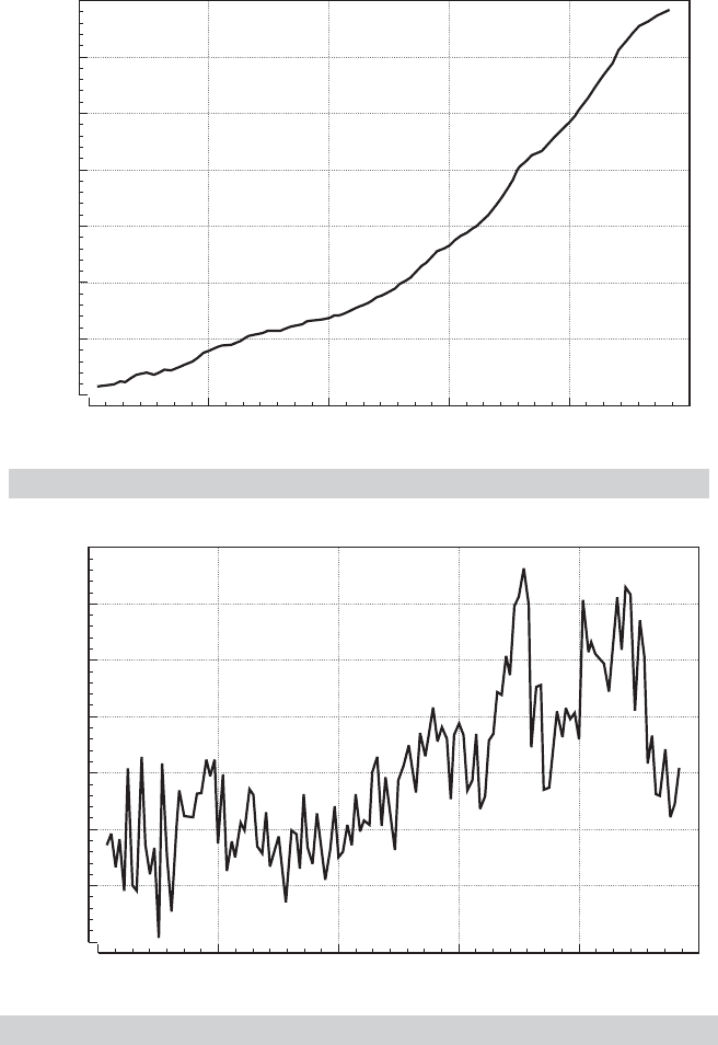
Example 21.1 A Nonstationary Series

The nominal GNP and price deﬂator variables in Appendix Table F21.1 are strongly trended,

so the mean is changing over time. Figures 21.1 through 21.3 plot the log of the GNP deﬂator

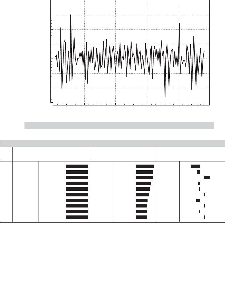
series in Table F21.1 and its ﬁrst and second differences. The original series and ﬁrst differ-

ences are obviously nonstationary, but the second differencing appears to have rendered the

series stationary.

The ﬁrst 10 autocorrelations of the log of the GNP deﬂator series are shown in Table 21.1.

The autocorrelations of the original series show the signature of a strongly trended, nonsta-

tionary series. The ﬁrst difference also exhibits nonstationarity, because the autocorrelations

are still very large after a lag of 10 periods. The second difference appears to be stationary,

with mild negative autocorrelation at the ﬁrst lag, but essentially none after that. Intuition

might suggest that further differencing would reduce the autocorrelation further, but that

would be incorrect. We leave as an exercise to show that, in fact, for values of γ less than

about 0.5, ﬁrst differencing of an AR(1) process actually increases autocorrelation.

There are yet further reﬁnements one might consider, such as removing seasonal effects from z

by differ-

encing by quarter or month. See Harvey (1990) and Davidson and MacKinnon (1993). Some recent work has

relaxed the assumption that d is an integer. The fractionally integrated series, or ARFIMA has been used to

model series in which the very long-run multipliers decay more slowly than would be predicted otherwise.

944

PART V

✦

Time Series and Macroeconometrics

Logprice

5.40

5.20

5.00

4.80

4.60

4.40

4.20

4.00

1950 1985

Quarter

1957 1964 1971 1978

FIGURE 21.1

Quarterly Data on log GNP Deﬂator.

d log p

0.0300

0.0250

0.0200

0.0150

0.0100

0.0050

0.0000

0.0050

1950 1985

Quarter

1957 1964 1971 1978

FIGURE 21.2

First Difference of log GNP Deﬂator.

21.2.2 RANDOM WALKS, TRENDS, AND SPURIOUS REGRESSIONS

In a seminal paper, Granger and Newbold (1974) argued that researchers had not paid

sufﬁcient attention to the warning of very high autocorrelation in the residuals from

conventional regression models. Among their conclusions were that macroeconomic

CHAPTER 21

✦

Nonstationary Data

945

log p

0.020

0.016

0.012

0.008

0.004

0.000

0.004

0.008

1950 1985

Quarter

1957 1964 1971 1978

FIGURE 21.3

Second Difference of log GNP Deﬂator.

TABLE 21.1

Autocorrelations for ln GNP Deﬂator

Autocorrelation Function Autocorrelation Function Autocorrelation Function

Lag Original Series, log Price First Difference of log Price Second Difference of log Price

1 1.000 0.812 −0.395

2 1.000 0.765 −0.112

3 0.999 0.776 0.258

4 0.999 0.682 −0.101

5 0.999 0.631 −0.022

6 0.998 0.592 0.076

7 0.998 0.523 −0.163

8 0.997 0.513 0.052

9 0.997 0.488 −0.054

10 0.997 0.491 0.062

data, as a rule, were integrated and that in regressions involving the levels of such data,

the standard signiﬁcance tests were usually misleading. The conventional t and F tests

would tend to reject the hypothesis of no relationship when, in fact, there might be none.

The general result at the center of these ﬁndings is that conventional linear regression,

ignoring serial correlation, of one random walk on another is virtually certain to sug-

gest a signiﬁcant relationship, even if the two are, in fact, independent. Among their

extreme conclusions, Granger and Newbold suggested that researchers use a critical t

value of 11.2 rather than the standard normal value of 1.96 to assess the signiﬁcance

of a coefﬁcient estimate. Phillips (1986) took strong issue with this conclusion. Based

on a more general model and on an analytical rather than a Monte Carlo approach,

he suggested that the normalized statistic t

√

T be used for testing purposes rather

than t

itself. For the 50 observations used by Granger and Newbold, the appropriate

946

PART V

✦

Time Series and Macroeconometrics

critical value would be close to 15! If anything, Granger and Newbold were too opti-

mistic.

The random walk with drift,

= μ + z

t−1

+ ε

, (21-1)

and the trend stationary process,

= μ + βt + ε

, (21-2)

where, in both cases, ε

is a white noise process, appear to be reasonable characteriza-

tions of many macroeconomic time series.

Clearly both of these will produce strongly

trended, nonstationary series,

so it is not surprising that regressions involving such

variables almost always produce signiﬁcant relationships. The strong correlation would

seem to be a consequence of the underlying trend, whether or not there really is any

regression at work. But Granger and Newbold went a step further. The intuition is less

clear if there is a pure random walk at work,

= z

t−1

+ ε

, (21-3)

but even here, they found that regression “relationships” appear to persist even in

unrelated series.

Each of these three series is characterized by a unit root. In each case, the data-

generating process (DGP) can be written

(1 − L)z

= α + v

, (21-4)

where α = μ, β, and 0, respectively, and v

is a stationary process. Thus, the characteristic

equation has a single root equal to one, hence the name. The upshot of Granger and

Newbold’s and Phillips’s ﬁndings is that the use of data characterized by unit roots has

the potential to lead to serious errors in inferences.

In all three settings, differencing or detrending would seem to be a natural ﬁrst step.

On the other hand, it is not going to be immediately obvious which is the correct way

to proceed—the data are strongly trended in all three cases—and taking the incorrect

approach will not necessarily improve matters. For example, ﬁrst differencing in (21-1)

or (21-3) produces a white noise series, but ﬁrst differencing in (21-2) trades the trend for

autocorrelation in the form of an MA(1) process. On the other hand, detrending—that

is, computing the residuals from a regression on time—is obviously counterproductive in

(21-1) and (21-3), even though the regression of z

on a trend will appear to be signiﬁcant

for the reasons we have been discussing, whereas detrending in (21-2) appears to be the

right approach.

Because none of these approaches is likely to be obviously preferable

The analysis to follow has been extended to more general disturbance processes, but that complicates

matters substantially. In this case, in fact, our assumption does cost considerable generality, but the extension

is beyond the scope of our work. Some references on the subject are Phillips and Perron (1988) and Davidson

and MacKinnon (1993).

The constant term μ produces the deterministic trend in the random walk with drift. For convenience,

suppose that the process starts at time zero. Then z



s=0

(μ + ε

) = μt +



s=0

. Thus, z

consists of

a deterministic trend plus a stochastic trend consisting of the sum of the innovations. The result is a variable

with increasing variance around a linear trend.

See Nelson and Kang (1984).

CHAPTER 21

✦

Nonstationary Data

947

at the outset, some means of choosing is necessary. Consider nesting all three models

in a single equation,

= μ + βt + z

t−1

+ ε

Now subtract z

t−1

from both sides of the equation and introduce the artiﬁcial parame-

ter γ .

− z

t−1

= μγ + βγt + (γ − 1)z

t−1

+ ε

= α

+ α

t + (γ − 1)z

t−1

+ ε

(21-5)

where, by hypothesis, γ = 1. Equation (21-5) provides the basis for a variety of tests

for unit roots in economic data. In principle, a test of the hypothesis that γ − 1 equals

zero gives conﬁrmation of the random walk with drift, because if γ equals 1 (and α

equals zero), then (21-1) results. If γ − 1 is less than zero, then the evidence favors

the trend stationary (or some other) model, and detrending (or some alternative) is

the preferable approach. The practical difﬁculty is that standard inference procedures

based on least squares and the familiar test statistics are not valid in this setting. The

issue is discussed in the next section.

21.2.3 TESTS FOR UNIT ROOTS IN ECONOMIC DATA

The implications of unit roots in macroeconomic data are, at least potentially, profound.

If a structural variable, such as real output, is truly I (1), then shocks to it will have per-

manent effects. If conﬁrmed, then this observation would mandate some rather serious

reconsideration of the analysis of macroeconomic policy. For example, the argument

that a change in monetary policy could have a transitory effect on real output would

vanish.

The literature is not without its skeptics, however. This result rests on a razor’s

edge. Although the literature is thick with tests that have failed to reject the hypothesis

that γ = 1, many have also not rejected the hypothesis that γ ≥ 0.95, and at 0.95 (or

even at 0.99), the entire issue becomes moot.

Consider the simple AR(1) model with zero-mean, white noise innovations,

= γ y

t−1

+ ε

The downward bias of the least squares estimator when γ approaches one has been

widely documented.

For |γ | < 1, however, the least squares estimator

c =



t=2

t−1



t=2

t−1

does have

plim c = γ

The 1980s saw the appearance of literally hundreds of studies, both theoretical and applied, of unit roots

in economic data. An important example is the seminal paper by Nelson and Plosser (1982). There is little

question but that this observation is an early part of the radical paradigm shift that has occurred in empirical

macroeconomics.

A large number of issues are raised in Maddala (1992, pp. 582–588).

See, for example, Evans and Savin (1981, 1984).

948

PART V

✦

Time Series and Macroeconometrics

and

√

T(c − γ)

−→ N[0, 1 − γ

Does the result hold up if γ =1? The case is called the unit root case, because in the

ARMA representation C(L)y

= ε

, the characteristic equation 1 −γ z = 0 has one root

equal to one. That the limiting variance appears to go to zero should raise suspicions.

The literature on the question dates back to Mann and Wald (1943) and Rubin (1950).

But for econometric purposes, the literature has a focal point at the celebrated papers

of Dickey and Fuller (1979, 1981). They showed that if γ equals one, then

T(c − γ)

−→ v,

where v is a random variable with ﬁnite, positive variance, and in ﬁnite samples,

E [c] < 1.

There are two important implications in the Dickey–Fuller results. First, the estima-

tor of γ is biased downward if γ equals one. Second, the OLS estimator of γ converges

to its probability limit more rapidly than the estimators to which we are accustomed.

That is, the variance of c under the null hypothesis is O(1/T

), not O(1/T). (In a

mean squared error sense, the OLS estimator is superconsistent.) It turns out that the

implications of this ﬁnding for the regressions with trended data are considerable.

We have already observed that in some cases, differencing or detrending is required

to achieve stationarity of a series. Suppose, though, that the preceding AR(1) model

is ﬁt to an I(1) series, despite that fact. The upshot of the preceding discussion is that

the conventional measures will tend to hide the true value of γ ; the sample estimate is

biased downward, and by dint of the very small true sampling variance, the conventional

t test will tend, incorrectly, to reject the hypothesis that γ = 1. The practical solution to

this problem devised by Dickey and Fuller was to derive, through Monte Carlo methods,

an appropriate set of critical values for testing the hypothesis that γ equals one in an

AR(1) regression when there truly is a unit root. One of their general results is that

the test may be carried out using a conventional t statistic, but the critical values for

the test must be revised: The standard t table is inappropriate. A number of variants

of this form of testing procedure have been developed. We will consider several of

them.

21.2.4 THE DICKEY–FULLER TESTS

The simplest version of the model to be analyzed is the random walk,

= γ y

t−1

+ ε

,ε

∼ N[0,σ

], and Cov[ε

,ε

] = 0 ∀t = s.

Under the null hypothesis that γ = 1, there are two approaches to carrying out the test.

The conventional t ratio

ˆγ − 1

Est. Std. Error( ˆγ)

A full derivation of this result is beyond the scope of this book. For the interested reader, a fairly compre-

hensive treatment at an accessible level is given in Chapter 17 of Hamilton (1994, pp. 475–542).