Greene W.H. Econometric Analysis
Подождите немного. Документ загружается.

CHAPTER 9
✦
The Generalized Regression Model
269
0246
Income
U
81012
2000
500
0
500
1000
1500
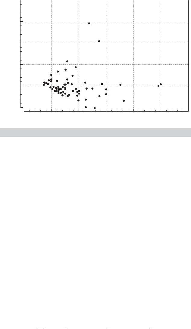
FIGURE 9.1
Plot of Residuals Against Income.
This makes the classical regression with homoscedastic disturbances a simple special
case with ω
i
= 1, i = 1,...,n. Intuitively, one might then think of the ω’s as weights
that are scaled in such a way as to reflect only the variety in the disturbance variances.
The scale factor σ
2
then provides the overall scaling of the disturbance process.
Example 9.1 Heteroscedastic Regression
The data in Appendix Table F7.3 give monthly credit card expenditure for 13,444 individuals.
Linear regression of monthly expenditure on a constant, age, income and its square, and a
dummy variable for home ownership using the 72 of the observations for which expenditure
was nonzero produces the residuals plotted in Figure 9.1. The pattern of the residuals is
characteristic of a regression with heteroscedasticity. (The subsample of 72 observations is
given in Appendix Table F9.1.)
We will examine the heteroscedastic regression model, first in general terms, then
with some specific forms of the disturbance covariance matrix. We begin by examining
the consequences of heteroscedasticity for least squares estimation. We then consider
robust estimation. Section 9.4.4 presents appropriate estimators of the asymptotic co-
variance matrix of the least squares estimator. Specification tests for heteroscedasticity
are considered in Section 9.5. Section 9.6 considers generalized (weighted) least squares,
which requires knowledge at least of the form of . Finally, two common applications
are examined in Section 9.7.
9.4.1 ORDINARY LEAST SQUARES ESTIMATION
We showed in Section 9.2 that in the presence of heteroscedasticity, the least squares
estimator b is still unbiased, consistent, and asymptotically normally distributed. The
asymptotic covariance matrix is
Asy. Var[b] =
σ
2
n
plim
1
n
X
X
−1
plim
1
n
X
X
plim
1
n
X
X
−1
. (9-18)

270
PART II
✦
Generalized Regression Model and Equation Systems
Estimation of the asymptotic covariance matrix would be based on
Var[b |X] = (X
X)
−1
σ
2
n
i=1
ω
i
x
i
x
i
(X
X)
−1
.
[See (9-5).] Assuming, as usual, that the regressors are well behaved, so that (X
X/n)
−1
converges to a positive definite matrix, we find that the mean square consistency of b
depends on the limiting behavior of the matrix:
Q
∗
n
=
X
X
n
=
1
n
n
i=1
ω
i
x
i
x
i
.
If Q
∗
n
converges to a positive definite matrix Q
∗
, then as n →∞, b will converge to β
in mean square. Under most circumstances, if ω
i
is finite for all i, then we would expect
this result to be true. Note that Q
∗
n
is a weighted sum of the squares and cross products
of x with weights ω
i
/n, which sum to 1. We have already assumed that another weighted
sum, X
X/n, in which the weights are 1/n, converges to a positive definite matrix Q,soit
would be surprising if Q
∗
n
did not converge as well. In general, then, we would expect that
b
a
∼
N
β,
σ
2
n
Q
−1
Q
∗
Q
−1
, with Q
∗
= plim Q
∗
n
.
A formal proof is based on Section 4.4 with Q
i
= ω
i
x
i
x
i
.
9.4.2 INEFFICIENCY OF ORDINARY LEAST SQUARES
It follows from our earlier results that b is inefficient relative to the GLS estimator. By
how much will depend on the setting, but there is some generality to the pattern. As
might be expected, the greater is the dispersion in ω
i
across observations, the greater
the efficiency of GLS over OLS. The impact of this on the efficiency of estimation will
depend crucially on the nature of the disturbance variances. In the usual cases, in which
ω
i
depends on variables that appear elsewhere in the model, the greater is the dispersion
in these variables, the greater will be the gain to using GLS. It is important to note,
however, that both these comparisons are based on knowledge of . In practice, one of
two cases is likely to be true. If we do have detailed knowledge of , the performance
of the inefficient estimator is a moot point. We will use GLS or feasible GLS anyway. In
the more common case, we will not have detailed knowledge of , so the comparison
is not possible.
9.4.3 THE ESTIMATED COVARIANCE MATRIX OF b
If the type of heteroscedasticity is known with certainty, then the ordinary least squares
estimator is undesirable; we should use generalized least squares instead. The precise
form of the heteroscedasticity is usually unknown, however. In that case, generalized
least squares is not usable, and we may need to salvage what we can from the results of
ordinary least squares.
The conventionally estimated covariance matrix for the least squares estimator
σ
2
(X
X)
−1
is inappropriate; the appropriate matrix is σ
2
(X
X)
−1
(X
X)(X
X)
−1
. It is
unlikely that these two would coincide, so the usual estimators of the standard errors
are likely to be erroneous. In this section, we consider how erroneous the conventional
estimator is likely to be.

CHAPTER 9
✦
The Generalized Regression Model
271
As usual,
s
2
=
e
e
n − K
=
ε
Mε
n − K
, (9-19)
where M = I −X(X
X)
−1
X
. Expanding this equation, we obtain
s
2
=
ε
ε
n − K
−
ε
X(X
X)
−1
X
ε
n − K
. (9-20)
Taking the two parts separately yields
E
ε
ε
n − K
*
*
*
*
X
=
trE [εε
|X]
n − K
=
nσ
2
n − K
. (9-21)
[We have used the scaling tr() = n.] In addition,
E
ε
X(X
X)
−1
X
ε
n − K
*
*
*
*
X
=
tr
E [(X
X)
−1
X
εε
X |X]
n − K
=
tr
σ
2
X
X
n
−1
X
X
n
n − K
=
σ
2
n − K
tr
X
X
n
−1
Q
∗
n
, (9-22)
where Q
∗
n
is defined after (9-18). As n →∞, the term in (9-21) will converge to σ
2
.
The term in (9-22) will converge to zero if b is consistent because both matrices in the
product are finite. Therefore;
If b is consistent, then lim
n→∞
E [s
2
] = σ
2
.
It can also be shown—we leave it as an exercise—that if the fourth moment of every
disturbance is finite and all our other assumptions are met, then
lim
n→∞
Var
e
e
n − K
= lim
n→∞
Var
ε
ε
n − K
= 0.
This result implies, therefore, that
If plim b = β, then plim s
2
= σ
2
.
Before proceeding, it is useful to pursue this result. The normalization tr() = n implies
that
σ
2
= ¯σ
2
=
1
n
i
σ
2
i
and ω
i
=
σ
2
i
¯σ
2
.
Therefore, our previous convergence result implies that the least squares estimator
s
2
converges to plim ¯σ
2
, that is, the probability limit of the average variance of the
disturbances, assuming that this probability limit exists. Thus, some further assumption
about these variances is necessary to obtain the result.
The difference between the conventional estimator and the appropriate (true) co-
variance matrix for b is
Est. Var[b |X] −Var[b |X] = s
2
(X
X)
−1
− σ
2
(X
X)
−1
(X
X)(X
X)
−1
. (9-23)

272
PART II
✦
Generalized Regression Model and Equation Systems
In a large sample (so that s
2
≈ σ
2
), this difference is approximately equal to
D =
σ
2
n
X
X
n
−1
X
X
n
−
X
X
n
X
X
n
−1
. (9-24)
The difference between the two matrices hinges on
=
X
X
n
−
X
X
n
=
n
i=1
1
n
x
i
x
i
−
n
i=1
ω
i
n
x
i
x
i
=
1
n
n
i=1
(1 − ω
i
)x
i
x
i
, (9-25)
where x
i
is the ith row of X. These are two weighted averages of the matrices Q
i
= x
i
x
i
,
using weights 1 for the first term and ω
i
for the second. The scaling tr() = n implies
that
i
(ω
i
/n) = 1. Whether the weighted average based on ω
i
/n differs much from the
one using 1/n depends on the weights. If the weights are related to the values in x
i
, then
the difference can be considerable. If the weights are uncorrelated with x
i
x
i
, however,
then the weighted average will tend to equal the unweighted average.
9
Therefore, the comparison rests on whether the heteroscedasticity is related to any
of x
k
or x
j
×x
k
. The conclusion is that, in general: If the heteroscedasticity is not correlated
with the variables in the model, then at least in large samples, the ordinary least squares
computations, although not the optimal way to use the data, will not be misleading.For
example, in the groupwise heteroscedasticity model of Section 9.7.2, if the observations
are grouped in the subsamples in a way that is unrelated to the variables in X, then the
usual OLS estimator of Var[b] will, at least in large samples, provide a reliable estimate
of the appropriate covariance matrix. It is worth remembering, however, that the least
squares estimator will be inefficient, the more so the larger are the differences among
the variances of the groups.
10
The preceding is a useful result, but one should not be overly optimistic. First, it
remains true that ordinary least squares is demonstrably inefficient. Second, if the pri-
mary assumption of the analysis—that the heteroscedasticity is unrelated to the vari-
ables in the model—is incorrect, then the conventional standard errors may be quite
far from the appropriate values.
9.4.4 ESTIMATING THE APPROPRIATE COVARIANCE MATRIX
FOR ORDINARY LEAST SQUARES
It is clear from the preceding that heteroscedasticity has some potentially serious im-
plications for inferences based on the results of least squares. The application of more
appropriate estimation techniques requires a detailed formulation of , however. It
may well be that the form of the heteroscedasticity is unknown. White (1980a) has
shown that it is still possible to obtain an appropriate estimator for the variance of the
least squares estimator, even if the heteroscedasticity is related to the variables in X.
9
Suppose, for example, that X contains a single column and that both x
i
and ω
i
are independent and identically
distributed random variables. Then x
x/n converges to E [x
2
i
], whereas x
x/n converges to Cov[ω
i
, x
2
i
] +
E [ω
i
]E [x
2
i
]. E [ω
i
] = 1, so if ω and x
2
are uncorrelated, then the sums have the same probability limit.
10
Some general results, including analysis of the properties of the estimator based on estimated variances,
are given in Taylor (1977).

CHAPTER 9
✦
The Generalized Regression Model
273
Referring to (9-18), we seek an estimator of
Q
∗
=
1
n
n
i=1
σ
2
i
x
i
x
i
.
White (1980a) shows that under very general conditions, the estimator
S
0
=
1
n
n
i=1
e
2
i
x
i
x
i
(9-26)
has
plim S
0
= plim Q
∗
.
11
We can sketch a proof of this result using the results we obtained in Section 4.4.
12
Note first that Q
∗
is not a parameter matrix in itself. It is a weighted sum of the outer
products of the rows of X (or Z for the instrumental variables case). Thus, we seek not to
“estimate” Q
∗
, but to find a function of the sample data that will be arbitrarily close to this
function of the population parameters as the sample size grows large. The distinction is
important. We are not estimating the middle matrix in (9-9) or (9-18); we are attempting
to construct a matrix from the sample data that will behave the same way that this matrix
behaves. In essence, if Q
∗
converges to a finite positive matrix, then we would be looking
for a function of the sample data that converges to the same matrix. Suppose that the true
disturbances ε
i
could be observed. Then each term in Q
∗
would equal E [ε
2
i
x
i
x
i
|x
i
]. With
some fairly mild assumptions about x
i
, then, we could invoke a law of large numbers
(see Theorems D.4 through D.9) to state that if Q
∗
has a probability limit, then
plim
1
n
n
i=1
σ
2
i
x
i
x
i
= plim
1
n
n
i=1
ε
2
i
x
i
x
i
.
The final detail is to justify the replacement of ε
i
with e
i
in S
0
. The consistency of b for
β is sufficient for the argument. (Actually, residuals based on any consistent estimator
of β would suffice for this estimator, but as of now, b or b
IV
is the only one in hand.)
The end result is that the White heteroscedasticity consistent estimator
Est. Asy. Var[b] =
1
n
1
n
X
X
−1
1
n
n
i=1
e
2
i
x
i
x
i
1
n
X
X
−1
= n(X
X)
−1
S
0
(X
X)
−1
(9-27)
can be used to estimate the asymptotic covariance matrix of b.
This result is extremely important and useful.
13
It implies that without actually
specifying the type of heteroscedasticity, we can still make appropriate inferences based
on the results of least squares. This implication is especially useful if we are unsure of
the precise nature of the heteroscedasticity (which is probably most of the time). We
will pursue some examples in Section 8.7.
11
See also Eicker (1967), Horn, Horn, and Duncan (1975), and MacKinnon and White (1985).
12
We will give only a broad sketch of the proof. Formal results appear in White (1980) and (2001).
13
Further discussion and some refinements may be found in Cragg (1982). Cragg shows how White’s obser-
vation can be extended to devise an estimator that improves on the efficiency of ordinary least squares.

274
PART II
✦
Generalized Regression Model and Equation Systems
TABLE 9.1
Least Squares Regression Results
Constant Age OwnRent Income Income
2
Sample mean 32.08 0.36 3.369
Coefficient −237.15 −3.0818 27.941 234.35 −14.997
Standard error 199.35 5.5147 82.922 80.366 7.4693
t ratio −1.19 −0.5590 0.337 2.916 −2.0080
White S.E. 212.99 3.3017 92.188 88.866 6.9446
D. and M. (1) 220.79 3.4227 95.566 92.122 7.1991
D. and M. (2) 221.09 3.4477 95.672 92.083 7.1995
R
2
= 0.243578, s = 284.75080
Mean expenditure =$262.53. Income is ×$10,000
Tests for heteroscedasticity: White =14.329,
Breusch–Pagan =41.920, Koenker–Bassett =6.187.
A number of studies have sought to improve on the White estimator for OLS.
14
The asymptotic properties of the estimator are unambiguous, but its usefulness in small
samples is open to question. The possible problems stem from the general result that
the squared OLS residuals tend to underestimate the squares of the true disturbances.
[That is why we use 1/(n − K) rather than 1/n in computing s
2
.] The end result is that in
small samples, at least as suggested by some Monte Carlo studies [e.g., MacKinnon and
White (1985)], the White estimator is a bit too optimistic; the matrix is a bit too small, so
asymptotic t ratios are a little too large. Davidson and MacKinnon (1993, p. 554) suggest
a number of fixes, which include (1) scaling up the end result by a factor n/(n − K) and
(2) using the squared residual scaled by its true variance, e
2
i
/m
ii
, instead of e
2
i
, where
m
ii
= 1 − x
i
(X
X)
−1
x
i
.
15
[See Exercise 9.6.b.] On the basis of their study, Davidson
and MacKinnon strongly advocate one or the other correction. Their admonition “One
should never use [the White estimator] because [(2)] always performs better” seems a bit
strong, but the point is well taken. The use of sharp asymptotic results in small samples
can be problematic. The last two rows of Table 9.1 show the recomputed standard errors
with these two modifications.
Example 9.2 The White Estimator
Using White’s estimator for the regression in Example 9.1 produces the results in the row
labeled “White S. E.” in Table 9.1. The two income coefficients are individually and jointly sta-
tistically significant based on the individual t ratios and F ( 2, 67) = [(0.244−0.064) /2]/[0.756/
(72− 5) ] = 7.976. The 1 percent critical value is 4.94.
The differences in the estimated standard errors seem fairly minor given the extreme
heteroscedasticity. One surprise is the decline in the standard error of the age coefficient.
The F test is no longer available for testing the joint significance of the two income coefficients
because it relies on homoscedasticity. A Wald test, however, may be used in any event. The
chi-squared test is based on
W = (Rb)
R
Est. Asy. Var[b]
R
−1
(Rb) where R =
00010
00001
,
14
See, e.g., MacKinnon and White (1985) and Messer and White (1984).
15
This is the standardized residual in (4-61). The authors also suggest a third correction, e
2
i
/m
2
ii
,asan
approximation to an estimator based on the “jackknife” technique, but their advocacy of this estimator
is much weaker than that of the other two.

CHAPTER 9
✦
The Generalized Regression Model
275
and the estimated asymptotic covariance matrix is the White estimator. The F statistic based
on least squares is 7.976. The Wald statistic based on the White estimator is 20.604; the
95 percent critical value for the chi-squared distribution with two degrees of freedom is 5.99,
so the conclusion is unchanged.
9.5 TESTING FOR HETEROSCEDASTICITY
Heteroscedasticity poses potentially severe problems for inferences based on least
squares. One can rarely be certain that the disturbances are heteroscedastic, however,
and unfortunately, what form the heteroscedasticity takes if they are. As such, it is use-
ful to be able to test for homoscedasticity and, if necessary, modify the estimation
procedures accordingly.
16
Several types of tests have been suggested. They can be
roughly grouped in descending order in terms of their generality and, as might be
expected, in ascending order in terms of their power.
17
We will examine the two most
commonly used tests.
Tests for heteroscedasticity are based on the following strategy. Ordinary least
squares is a consistent estimator of β even in the presence of heteroscedasticity. As such,
the ordinary least squares residuals will mimic, albeit imperfectly because of sampling
variability, the heteroscedasticity of the true disturbances. Therefore, tests designed
to detect heteroscedasticity will, in general, be applied to the ordinary least squares
residuals.
9.5.1 WHITE’S GENERAL TEST
To formulate most of the available tests, it is necessary to specify, at least in rough
terms, the nature of the heteroscedasticity. It would be desirable to be able to test a
general hypothesis of the form
H
0
: σ
2
i
= σ
2
for all i,
H
1
: Not H
0
.
In view of our earlier findings on the difficulty of estimation in a model with n unknown
parameters, this is rather ambitious. Nonetheless, such a test has been suggested by
White (1980b). The correct covariance matrix for the least squares estimator is
Var[b |X] = σ
2
[X
X]
−1
[X
X][X
X]
−1
,
which, as we have seen, can be estimated using (9-27). The conventional estimator is
V = s
2
[X
X]
−1
. If there is no heteroscedasticity, then V will give a consistent estimator
of Var[b |X], whereas if there is, then it will not. White has devised a statistical test based
on this observation. A simple operational version of his test is carried out by obtaining
nR
2
in the regression of e
2
i
on a constant and all unique variables contained in x and
16
There is the possibility that a preliminary test for heteroscedasticity will incorrectly lead us to use weighted
least squares or fail to alert us to heteroscedasticity and lead us improperly to use ordinary least squares.
Some limited results on the properties of the resulting estimator are given by Ohtani and Toyoda (1980).
Their results suggest that it is best to test first for heteroscedasticity rather than merely to assume that it is
present.
17
A study that examines the power of several tests for heteroscedasticity is Ali and Giaccotto (1984).

276
PART II
✦
Generalized Regression Model and Equation Systems
all the squares and cross products of the variables in x. The statistic is asymptotically
distributed as chi-squared with P − 1 degrees of freedom, where P is the number of
regressors in the equation, including the constant.
The White test is extremely general. To carry it out, we need not make any specific
assumptions about the nature of the heteroscedasticity. Although this characteristic is
a virtue, it is, at the same time, a potentially serious shortcoming. The test may reveal
heteroscedasticity, but it may instead simply identify some other specification error
(such as the omission of x
2
from a simple regression).
18
Except in the context of a
specific problem, little can be said about the power of White’s test; it may be very low
against some alternatives. In addition, unlike some of the other tests we shall discuss,
the White test is nonconstructive. If we reject the null hypothesis, then the result of the
test gives no indication of what to do next.
9.5.2 THE BREUSCH–PAGAN/GODFREY LM TEST
Breusch and Pagan
19
have devised a Lagrange multiplier test of the hypothesis that
σ
2
i
= σ
2
f (α
0
+ α
z
i
), where z
i
is a vector of independent variables.
20
The model is
homoscedastic if α = 0. The test can be carried out with a simple regression:
LM =
1
2
explained sum of squares in the regression of e
2
i
/(e
e/n) on z
i
.
For computational purposes, let Z be the n × P matrix of observations on (1, z
i
), and
let g be the vector of observations of g
i
= e
2
i
/(e
e/n) − 1. Then
LM =
1
2
[g
Z(Z
Z)
−1
Z
g]. (9-28)
Under the null hypothesis of homoscedasticity, LM has a limiting chi-squared distribu-
tion with degrees of freedom equal to the number of variables in z
i
. This test can be
applied to a variety of models, including, for example, those examined in Example 9.3 (2)
and in Sections 9.7.1 and 9.7.2.
21
It has been argued that the Breusch–Pagan Lagrange multiplier test is sensitive to
the assumption of normality. Koenker (1981) and Koenker and Bassett (1982) suggest
that the computation of LM be based on a more robust estimator of the variance of ε
2
i
,
V =
1
n
n
i=1
e
2
i
−
e
e
n
2
.
The variance of ε
2
i
is not necessarily equal to 2σ
4
if ε
i
is not normally distributed. Let u
equal (e
2
1
, e
2
2
,...,e
2
n
) and i be an n × 1 column of 1s. Then ¯u = e
e/n. With this change,
the computation becomes
LM =
1
V
(u − ¯u i)
Z(Z
Z)
−1
Z
(u − ¯u i).
18
Thursby (1982) considers this issue in detail.
19
Breusch and Pagan (1979).
20
Lagrange multiplier tests are discussed in Section 14.6.3.
21
The model σ
2
i
=σ
2
exp(α
z
i
) is one of these cases. In analyzing this model specifically, Harvey (1976)
derived the same test statistic.

CHAPTER 9
✦
The Generalized Regression Model
277
Under normality, this modified statistic will have the same limiting distribution as the
Breusch–Pagan statistic, but absent normality, there is some evidence that it provides a
more powerful test. Waldman (1983) has shown that if the variables in z
i
are the same
as those used for the White test described earlier, then the two tests are algebraically
the same.
Example 9.3 Testing for Heteroscedasticity
1. White’s Test: For the data used in Example 9.1, there are 15 variables in x⊗x including the
constant term. But since Ownrent
2
=OwnRent and Income ×Income =Income
2
, only 13 are
unique. Regression of the squared least squares residuals on these 13 variables produces
R
2
= 0.199013. The chi-squared statistic is therefore 72(0.199013) = 14.329. The 95 percent
critical value of chi-squared with 12 degrees of freedom is 21.03, so despite what might seem
to be obvious in Figure 9.1, the hypothesis of homoscedasticity is not rejected by this test.
2. Breusch–Pagan Test: This test requires a specific alternative hypothesis. For this pur-
pose, we specify the test based on z =[1, Income, Income
2
]. Using the least squares resid-
uals, we compute g
i
= e
2
i
/(e
e/72) − 1; then LM =
1
2
g
Z(Z
Z)
−1
Z
g. The sum of squares
is 5,432,562.033. The computation produces LM = 41.920. The critical value for the chi-
squared distribution with two degrees of freedom is 5.99, so the hypothesis of homoscedas-
ticity is rejected. The Koenker and Bassett variant of this statistic is only 6.187, which is still
significant but much smaller than the LM statistic. The wide difference between these two
statistics suggests that the assumption of normality is erroneous. Absent any knowledge
of the heteroscedasticity, we might use the Bera and Jarque (1981, 1982) and Kiefer and
Salmon (1983) test for normality,
χ
2
[2] = n[1/6(m
3
/s
3
)
2
+ 1/25(( m
4
− 3)/s
4
)
2
]
where m
j
=(1/n)
i
e
j
i
. Under the null hypothesis of homoscedastic and normally distributed
disturbances, this statistic has a limiting chi-squared distribution with two degrees of free-
dom. Based on the least squares residuals, the value is 497.35, which certainly does lead
to rejection of the hypothesis. Some caution is warranted here, however. It is unclear what
part of the hypothesis should be rejected. We have convincing evidence in Figure 9.1 that
the disturbances are heteroscedastic, so the assumption of homoscedasticity underlying
this test is questionable. This does suggest the need to examine the data before applying a
specification test such as this one.
9.6 WEIGHTED LEAST SQUARES
Having tested for and found evidence of heteroscedasticity, the logical next step is to
revise the estimation technique to account for it. The GLS estimator is
ˆ
β = (X
−1
X)
−1
X
−1
y. (9-29)
Consider the most general case, Var[ε
i
|X] = σ
2
i
= σ
2
ω
i
. Then
−1
is a diagonal matrix
whose ith diagonal element is 1/ω
i
. The GLS estimator is obtained by regressing
Py =
⎡
⎢
⎢
⎢
⎢
⎣
y
1
/
√
ω
1
y
2
/
√
ω
2
.
.
.
y
n
/
√
ω
n
⎤
⎥
⎥
⎥
⎥
⎦
on PX =
⎡
⎢
⎢
⎢
⎢
⎣
x
1
/
√
ω
1
x
2
/
√
ω
2
.
.
.
x
n
/
√
ω
n
⎤
⎥
⎥
⎥
⎥
⎦
.

278
PART II
✦
Generalized Regression Model and Equation Systems
Applying ordinary least squares to the transformed model, we obtain the weighted least
squares (WLS) estimator.
ˆ
β =
n
i=1
w
i
x
i
x
i
−1
n
i=1
w
i
x
i
y
i
,
where w
i
=1/ω
i
.
22
The logic of the computation is that observations with smaller vari-
ances receive a larger weight in the computations of the sums and therefore have greater
influence in the estimates obtained.
9.6.1 WEIGHTED LEAST SQUARES WITH KNOWN
A common specification is that the variance is proportional to one of the regressors
or its square. Our earlier example of family expenditures is one in which the relevant
variable is usually income. Similarly, in studies of firm profits, the dominant variable is
typically assumed to be firm size. If
σ
2
i
= σ
2
x
2
ik
,
then the transformed regression model for GLS is
y
x
k
= β
k
+ β
1
x
1
x
k
+ β
2
x
2
x
k
+···+
ε
x
k
. (9-30)
If the variance is proportional to x
k
instead of x
2
k
, then the weight applied to each
observation is 1/
√
x
k
instead of 1/x
k
.
In (9-30), the coefficient on x
k
becomes the constant term. But if the variance is
proportional to any power of x
k
other than two, then the transformed model will no
longer contain a constant, and we encounter the problem of interpreting R
2
mentioned
earlier. For example, no conclusion should be drawn if the R
2
in the regression of y/z on
1/z and x/z is higher than in the regression of y on a constant and x for any z, including
x. The good fit of the weighted regression might be due to the presence of 1/z on both
sides of the equality.
It is rarely possible to be certain about the nature of the heteroscedasticity in a
regression model. In one respect, this problem is only minor. The weighted least squares
estimator
ˆ
β =
n
i=1
w
i
x
i
x
i
−1
n
i=1
w
i
x
i
y
i
is consistent regardless of the weights used, as long as the weights are uncorrelated with
the disturbances.
But using the wrong set of weights has two other consequences that may be less
benign. First, the improperly weighted least squares estimator is inefficient. This point
might be moot if the correct weights are unknown, but the GLS standard errors will
22
The weights are often denoted w
i
=1/σ
2
i
. This expression is consistent with the equivalent
ˆ
β =[X
(σ
2
)
−1
X]
−1
X
(σ
2
)
−1
y.Theσ
2
’s cancel, leaving the expression given previously.