Greene W.H. Econometric Analysis
Подождите немного. Документ загружается.


CHAPTER 9
✦
The Generalized Regression Model
279
also be incorrect. The asymptotic covariance matrix of the estimator
ˆ
β = [X
V
−1
X]
−1
X
V
−1
y (9-31)
is
Asy. Var[
ˆ
β] = σ
2
[X
V
−1
X]
−1
X
V
−1
V
−1
X[X
V
−1
X]
−1
. (9-32)
This result may or may not resemble the usual estimator, which would be the matrix in
brackets, and underscores the usefulness of the White estimator in (9-27).
The standard approach in the literature is to use OLS with the White estimator
or some variant for the asymptotic covariance matrix. One could argue both flaws and
virtues in this approach. In its favor, robustness to unknown heteroscedasticity is a
compelling virtue. In the clear presence of heteroscedasticity, however, least squares
can be extremely inefficient. The question becomes whether using the wrong weights is
better than using no weights at all. There are several layers to the question. If we use
one of the models mentioned earlier—Harvey’s, for example, is a versatile and flexible
candidate—then we may use the wrong set of weights and, in addition, estimation of
the variance parameters introduces a new source of variation into the slope estimators
for the model. A heteroscedasticity robust estimator for weighted least squares can
be formed by combining (9-32) with the White estimator. The weighted least squares
estimator in (9-31) is consistent with any set of weights V =diag[v
1
,v
2
,...,v
n
]. Its
asymptotic covariance matrix can be estimated with
Est. Asy. Var[
ˆ
β] = (X
V
−1
X)
−1
n
i=1
e
2
i
v
2
i
x
i
x
i
(X
V
−1
X)
−1
. (9-33)
Any consistent estimator can be used to form the residuals. The weighted least squares
estimator is a natural candidate.
9.6.2 ESTIMATION WHEN
CONTAINS UNKNOWN PARAMETERS
The general form of the heteroscedastic regression model has too many parameters to
estimate by ordinary methods. Typically, the model is restricted by formulating σ
2
as
a function of a few parameters, as in σ
2
i
= σ
2
x
α
i
or σ
2
i
= σ
2
(x
i
α)
2
. Write this as (α).
FGLS based on a consistent estimator of (α) (meaning a consistent estimator of α)
is asymptotically equivalent to full GLS. The new problem is that we must first find
consistent estimators of the unknown parameters in (α). Two methods are typically
used, two-step GLS and maximum likelihood. We consider the two-step estimator here
and the maximum likelihood estimator in Chapter 14.
For the heteroscedastic model, the GLS estimator is
ˆ
β =
n
i=1
1
σ
2
i
x
i
x
i
−1
n
i=1
1
σ
2
i
x
i
y
i
. (9-34)
The two-step estimators are computed by first obtaining estimates ˆσ
2
i
, usually using some
function of the ordinary least squares residuals. Then,
ˆ
ˆ
β uses (9-34) and ˆσ
2
i
. The ordinary
least squares estimator of β, although inefficient, is still consistent. As such, statistics
computed using the ordinary least squares residuals, e
i
= (y
i
−x
i
b), will have the same
asymptotic properties as those computed using the true disturbances, ε
i
= (y
i
− x
i
β).

280
PART II
✦
Generalized Regression Model and Equation Systems
This result suggests a regression approach for the true disturbances and variables z
i
that
may or may not coincide with x
i
. Now E [ε
2
i
|z
i
] = σ
2
i
,so
ε
2
i
= σ
2
i
+ v
i
,
where v
i
is just the difference between ε
2
i
and its conditional expectation. Because ε
i
is
unobservable, we would use the least squares residual, for which e
i
= ε
i
− x
i
(b − β) =
ε
i
+ u
i
. Then, e
2
i
= ε
2
i
+ u
2
i
+ 2ε
i
u
i
. But, in large samples, as b
p
−→ β, terms in u
i
will
become negligible, so that at least approximately,
23
e
2
i
= σ
2
i
+ v
∗
i
.
The procedure suggested is to treat the variance function as a regression and use
the squares or some other functions of the least squares residuals as the dependent
variable.
24
For example, if σ
2
i
= z
i
α, then a consistent estimator of α will be the least
squares slopes, a, in the “model,”
e
2
i
= z
i
α + v
∗
i
.
In this model, v
∗
i
is both heteroscedastic and autocorrelated, so a is consistent but
inefficient. But, consistency is all that is required for asymptotically efficient estimation
of β using ( ˆα). It remains to be settled whether improving the estimator of α in this
and the other models we will consider would improve the small sample properties of
the two-step estimator of β.
25
The two-step estimator may be iterated by recomputing the residuals after comput-
ing the FGLS estimates and then reentering the computation. The asymptotic properties
of the iterated estimator are the same as those of the two-step estimator, however. In
some cases, this sort of iteration will produce the maximum likelihood estimator at
convergence. Yet none of the estimators based on regression of squared residuals on
other variables satisfy the requirement. Thus, iteration in this context provides little
additional benefit, if any.
9.7 APPLICATIONS
This section will present two common applications of the heteroscedastic regression
model, Harvey’s model of multiplicative heteroscedasticity and a model of groupwise
heteroscedasticity that extends to the disturbance variance some concepts that are usu-
ally associated with variation in the regression function.
9.7.1 MULTIPLICATIVE HETEROSCEDASTICITY
Harvey’s (1976) model of multiplicative heteroscedasticity is a very flexible, general
model that includes most of the useful formulations as special cases. The general for-
mulation is
σ
2
i
= σ
2
exp(z
i
α).
23
See Amemiya (1985) and Harvey (1976) for formal analyses.
24
See, for example, Jobson and Fuller (1980).
25
Fomby, Hill, and Johnson (1984, pp. 177–186) and Amemiya (1985, pp. 203–207; 1977a) examine this model.
CHAPTER 9
✦
The Generalized Regression Model
281
A model with heteroscedasticity of the form
σ
2
i
= σ
2
M
3
m=1
z
α
m
im
results if the logs of the variables are placed in z
i
. The groupwise heteroscedasticity
model described in Example 9.4 is produced by making z
i
a set of group dummy vari-
ables (one must be omitted). In this case, σ
2
is the disturbance variance for the base
group whereas for the other groups, σ
2
g
= σ
2
exp(α
g
).
Example 9.4 Multiplicative Heteroscedasticity
In Example 6.4, we fit a cost function for the U.S. airline industry of the form
In C
it
= β
1
+ β
2
In Q
it
+ β
3
(lnQ
it
)
2
+ β
4
ln P
fuel,i,t
+ β
5
Loadfactor
i,t
+ ε
i,t
where C
i,t
is total cost, Q
i,t
is output, and P
fuel,i,t
is the price of fuel and the 90 observations
in the data set are for six firms observed for 15 years. (The model also included dummy
variables for firm and year, which we will omit for simplicity.) We now consider a revised
model in which the load factor appears in the variance of ε
i,t
rather than in the regression
function. The model is
σ
2
i,t
= σ
2
exp(γ Loadfactor
i,t
)
= exp(γ
1
+ γ
2
Loadfactor
i,t
).
The constant in the implied regression is γ
1
= ln σ
2
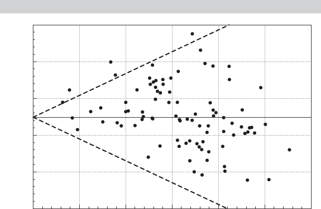
. Figure 9.2 shows a plot of the least
squares residuals against Load factor for the 90 observations. The figure does suggest the
presence of heteroscedasticity. (The dashed lines are placed to highlight the effect.) We
computed the LM statistic using (9-28). The chi-squared statistic is 2.959. This is smaller
than the critical value of 3.84 for one degree of freedom, so on this basis, the null hypothesis
of homoscedasticity with respect to the load factor is not rejected.
FIGURE 9.2
Plot of Residuals Against Load Factor.
0.400
0.40
0.24
0.08
e
0.08
0.24
0.40
0.450 0.500 0.550
Load Factor
0.600 0.650 0.700

282
PART II
✦
Generalized Regression Model and Equation Systems
TABLE 9.2
Multiplicative Heteroscedasticity Model
Constant Ln Q Ln
2
Q Ln P
f
R
2
Sum of Squares
OLS 9.1382 0.92615 0.029145 0.41006
0.24507
a
0.032306 0.012304 0.018807 0.9861674
c
1.577479
d
0.22595
b
0.030128 0.011346 0.017524
Two step 9.2463 0.92136 0.024450 0.40352
0.21896 0.033028 0.011412 0.016974
0.986119 1.612938
Iterated
e
9.2774 0.91609 0.021643 0.40174
0.20977 0.032993 0.011017 0.016332
0.986071 1.645693
a
Conventional OLS standard errors
b
White robust standard errors
c
Squared correlation between actual and fitted values
d
Sum of squared residuals
e
Values of c
2
by iteration: 8.254344, 11.622473, 11.705029, 11.710618, 11.711012, 11.711040, 11.711042
To begin, we use OLS to estimate the parameters of the cost function and the set of
residuals, e
i,t
. Regression of log(e
2
it
) on a constant and the load factor provides estimates of
γ
1
and γ
2
, denoted c
1
and c
2
. The results are shown in Table 9.2. As Harvey notes, exp( c
1
)
does not necessarily estimate σ
2
consistently—for normally distributed disturbances, it is
low by a factor of 1.2704. However, as seen in (9-29), the estimate of σ
2
(biased or otherwise)
is not needed to compute the FGLS estimator. Weights w
i,t
= exp( −c
1
−c
2
Loadfactor
i,t
)are
computed using these estimates, then weighted least squares using (9-30) is used to obtain
the FGLS estimates of β. The results of the computations are shown in Table 9.2.
We might consider iterating the procedure. Using the results of FGLS at step 2, we can
recompute the residuals, then recompute c
1
and c
2
and the weights, and then reenter the
iteration. The process converges when the estimate of c
2
stabilizes. This requires seven iter-
ations. The results are shown in Table 9.2. As noted earlier, iteration does not produce any
gains here. The second step estimator is already fully efficient. Moreover, this does not pro-
duce the MLE, either. That would be obtained by regressing [e
2
i,t
/exp(c
1
+c
2
Loadfactor
i,t
) −1]
on the constant and load factor at each iteration to obtain the new estimates. We will revisit
this in Chapter 14.
9.7.2 GROUPWISE HETEROSCEDASTICITY
A groupwise heteroscedastic regression has the structural equations
y
i
= x
i
β + ε
i
, i = 1,...,n,
E [ε
i
|x
i
] = 0, i = 1,...,n.
The n observations are grouped into G groups, each with n
g
observations. The slope
vector is the same in all groups, but within group g
Var[ε
ig
|x
ig
] = σ
2
g
, i = 1,...,n
g
.
If the variances are known, then the GLS estimator is
ˆ
β =
⎡
⎣
G
g=1
1
σ
2
g
X
g
X
g
⎤
⎦
−1
⎡
⎣
G
g=1
1
σ
2
g
X
g
y
g
⎤
⎦
. (9-35)

CHAPTER 9
✦
The Generalized Regression Model
283
Because X
g
y
g
= X
g
X
g
b
g
, where b
g
is the OLS estimator in the gth subset of observa-
tions,
ˆ
β =
⎡
⎣
G
g=1
1
σ
2
g
X
g
X
g
⎤
⎦
−1
⎡
⎣
G
g=1
1
σ
2
g
X
g
X
g
b
g
⎤
⎦
=
⎡
⎣
G
g=1
V
g
⎤
⎦
−1
⎡
⎣
G
g=1
V
g
b
g
⎤
⎦
=
G
g=1
W
g
b
g
.
This result is a matrix weighted average of the G least squares estimators. The weighting
matrices are W
g
=
G
g=1
Var[b
g
]
−1
−1
Var[b
g
]
−1
. The estimator with the smaller
covariance matrix therefore receives the larger weight. (If X
g
is the same in every group,
then the matrix W
g
reduces to the simple, w
g
I = (h
g
/
g
h
g
)I where h
g
= 1/σ
2
g
.)
The preceding is a useful construction of the estimator, but it relies on an algebraic
result that might be unusable. If the number of observations in any group is smaller than
the number of regressors, then the group specific OLS estimator cannot be computed.
But, as can be seen in (9-35), that is not what is needed to proceed; what is needed are
the weights. As always, pooled least squares is a consistent estimator, which means that
using the group specific subvectors of the OLS residuals,
ˆσ
2
g
=
e
g
e
g
n
g
, (9-36)
provides the needed estimator for the group specific disturbance variance. Thereafter,
(9-35) is the estimator and the inverse matrix in that expression gives the estimator of
the asymptotic covariance matrix.
Continuing this line of reasoning, one might consider iterating the estimator by re-
turning to (9-36) with the two-step FGLS estimator, recomputing the weights, then
returning to (9-35) to recompute the slope vector. This can be continued until conver-
gence. It can be shown [see Oberhofer and Kmenta (1974)] that so long as (9-36) is used
without a degrees of freedom correction, then if this does converge, it will do so at the
maximum likelihood estimator (with normally distributed disturbances).
For testing the homoscedasticity assumption, both White’s test and the LM test are
straightforward. The variables thought to enter the conditional variance are simply a set
of G − 1 group dummy variables, not including one of them (to avoid the dummy vari-
able trap), which we’ll denote Z
∗
. Because the columns of Z
∗
are binary and orthogonal,
to carry out White’s test, we need only regress the squared least squares residuals on a
constant and Z
∗
and compute NR
2
where N =
g
n
g
. The LM test is also straightfor-
ward. For purposes of this application of the LM test, it will prove convenient to replace
the overall constant in Z in (9-28), with the remaining group dummy variable. Since the
column space of the full set of dummy variables is the same as that of a constant and
G−1 of them, all results that follow will be identical. In (9-28), the vector g will now be
G subvectors where each subvector is the n
g
elements of [(e
2
ig
/ ˆσ
2
) −1], and ˆσ
2
= e
e/N.
By multiplying it out, we find that g
Z is the G vector with elements n
g
[( ˆσ
2
g
/ ˆσ
2
) − 1],
while (Z
Z)
−1
is the G × G matrix with diagonal elements 1/n
g
. It follows that
LM =
1
2
g
Z(Z
Z)
−1
Z
g =
1
2
G
g=1
n
g
ˆσ
2
g
ˆσ
2
− 1
2
. (9-37)
Both statistics have limiting chi squared distributions with G − 1 degrees of freedom
under the null hypothesis of homoscedasticity. (There are only G−1 degrees of freedom
because the hypothesis imposes G − 1 restrictions, that the G variances are all equal to
each other. Implicitly, one of the variances is free and the other G − 1 equal that one.)
284
PART II
✦
Generalized Regression Model and Equation Systems
Example 9.5 Groupwise Heteroscedasticity
Baltagi and Griffin (1983) is a study of gasoline usage in 18 of the 30 OECD countries. The
model analyzed in the paper is
ln (Gasoline usage/car)
i,t
= β
1
+ β
2
ln(Per capita income)
i,t
+ β
3
ln Price
i,t
β
4
ln(Cars per capita)
i,t
+ ε
i,t
,
where i = country and t = 1960, ..., 1978. This is a balanced panel (see Section 9.2) with
19(18) = 342 observations in total. The data are given in Appendix Table F9.2.
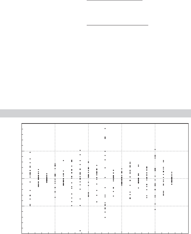
Figure 9.3 displays the OLS residuals using the least squares estimates of the model
above with the addition of 18 country dummy variables (1 to 18) (and without the overall con-
stant). (The country dummy variables are used so that the country-specific residuals will have
mean zero). The F statistic for testing the null hypothesis that all the constants are equal is
F
( G − 1) ,
g
n
g
− K − G
=
(e
0
e
0
− e
1
e
1
)/( G − 1)
(e
1
e
1
/
g
n
g
− K − G)
=
(14.90436 − 2.73649) /17
2.73649/(342 − 3 − 18)
= 83.960798,
where e
0
is the vector of residuals in the regression with a single constant term and e
1
is the
regression with country specific constant terms. The critical value from the F table with 17
and 321 degrees of freedom is 1.655. The regression results are given in Table 9.3. Figure 9.3
does convincingly suggest the presence of groupwise heteroscedasticity. The White and LM
statistics are 342( 0.38365) = 131.21 and 279.588, respectively. The critical value from the
chi-squared distribution with 17 degrees of freedom is 27.587. So, we reject the hypothesis
of homoscedasticity and proceed to fit the model by feasible GLS. The two-step estimators
are shown in Table 9.3. The FGLS estimator is computed by using weighted least squares,
where the weights are 1/ ˆσ
2
g
for each observation in country g. Comparing the White standard
errors to the two-step estimators, we see that in this instance, there is a substantial gain to
using feasible generalized least squares.
FIGURE 9.3
Plot of OLS Residuals by Country.
Country
0.20
0.00
0.20
0.40
0.40
4 8 12 16 200
Least Squares Residual

CHAPTER 9
✦
The Generalized Regression Model
285
TABLE 9.3
Estimated Gasoline Consumption Equations
OLS FGLS
Coefficient Std. Error White Std. Err. Coefficient Std. Error
In Income 0.66225 0.07339 0.07277 0.57507 0.02927
In Price −0.32170 0.04410 0.05381 −0.27967 0.03519
Cars/Cap. −0.64048 0.02968 0.03876 −0.56540 0.01613
Country 1 2.28586 0.22832 0.22608 2.43707 0.11308
Country 2 2.16555 0.21290 0.20983 2.31699 0.10225
Country 3 3.04184 0.21864 0.22479 3.20652 0.11663
Country 4 2.38946 0.20809 0.20783 2.54707 0.10250
Country 5 2.20477 0.21647 0.21087 2.33862 0.10101
Country 6 2.14987 0.21788 0.21846 2.30066 0.10893
Country 7 2.33711 0.21488 0.21801 2.57209 0.11206
Country 8 2.59233 0.24369 0.23470 2.72376 0.11384
Country 9 2.23255 0.23954 0.22973 2.34805 0.10795
Country 10 2.37593 0.21184 0.22643 2.58988 0.11821
Country 11 2.23479 0.21417 0.21311 2.39619 0.10478
Country 12 2.21670 0.20304 0.20300 2.38486 0.09950
Country 13 1.68178 0.16246 0.17133 1.90306 0.08146
Country 14 3.02634 0.39451 0.39180 3.07825 0.20407
Country 15 2.40250 0.22909 0.23280 2.56490 0.11895
Country 16 2.50999 0.23566 0.26168 2.82345 0.13326
Country 17 2.34545 0.22728 0.22322 2.48214 0.10955
Country 18 3.05525 0.21960 0.22705 3.21519 0.11917
9.8 SUMMARY AND CONCLUSIONS
This chapter has introduced a major extension of the classical linear model. By allowing
for heteroscedasticity and autocorrelation in the disturbances, we expand the range
of models to a large array of frameworks. We will explore these in the next several
chapters. The formal concepts introduced in this chapter include how this extension
affects the properties of the least squares estimator, how an appropriate estimator
of the asymptotic covariance matrix of the least squares estimator can be computed
in this extended modeling framework and, finally, how to use the information about
the variances and covariances of the disturbances to obtain an estimator that is more
efficient than ordinary least squares.
We have analyzed in detail one form of the generalized regression model, the model
of heteroscedasticity. We first considered least squares estimation. The primary result
for least squares estimation is that it retains its consistency and asymptotic normality,
but some correction to the estimated asymptotic covariance matrix may be needed for
appropriate inference. The White estimator is the standard approach for this compu-
tation. After examining two general tests for heteroscedasticity, we then narrowed the
model to some specific parametric forms, and considered weighted (generalized) least
squares for efficient estimation and maximum likelihood estimation. If the form of the
heteroscedasticity is known but involves unknown parameters, then it remains uncer-
tain whether FGLS corrections are better than OLS. Asymptotically, the comparison is
clear, but in small or moderately sized samples, the additional variation incorporated
by the estimated variance parameters may offset the gains to GLS.

286
PART II
✦
Generalized Regression Model and Equation Systems
Key Terms and Concepts
•
Aitken’s theorem
•
Asymptotic properties
•
Autocorrelation
•
Breusch–Pagan Lagrange
multiplier test
•
Efficient estimator
•
Feasible generalized least
squares (FGLS)
•
Finite-sample properties
•
Generalized least squares
(GLS)
•
Generalized linear
regression model
•
Generalized sum of squares
•
Groupwise
heteroscedasticity
•
Heteroscedasticity
•
Kruskal’s theorem
•
Lagrange multiplier test
•
Multiplicative
heteroscedasticity
•
Nonconstructive test
•
Ordinary least squares
(OLS)
•
Panel data
•
Parametric model
•
Robust estimation
•
Robust estimator
•
Robustness to unknown
heteroscedasticity
•
Semiparametric model
•
Specification test
•
Spherical disturbances
•
Two-step estimator
•
Wald test
•
Weighted least squares
(WLS)
•
White heteroscedasticity
consistent estimator
•
White test
Exercises
1. What is the covariance matrix, Cov[
ˆ
β,
ˆ
β −b], of the GLS estimator
ˆ
β =
(X
−1
X)
−1
X
−1
y and the difference between it and the OLS estimator, b =
(X
X)
−1
X
y? The result plays a pivotal role in the development of specification
tests in Hausman (1978).
2. This and the next two exercises are based on the test statistic usually used to test a
set of J linear restrictions in the generalized regression model
F[J, n − K] =
(R
ˆ
β − q)
[R(X
−1
X)
−1
R
]
−1
(R
ˆ
β − q)/J
(y − X
ˆ
β)
−1
(y − X
ˆ
β)/(n − K)
,
where
ˆ
β is the GLS estimator. Show that if is known, if the disturbances are
normally distributed and if the null hypothesis, Rβ = q, is true, then this statistic
is exactly distributed as F with J and n − K degrees of freedom. What assump-
tions about the regressors are needed to reach this conclusion? Need they be non-
stochastic?
3. Now suppose that the disturbances are not normally distributed, although is still
known. Show that the limiting distribution of previous statistic is (1/ J) times a chi-
squared variable with J degrees of freedom. (Hint: The denominator converges to
σ
2
.) Conclude that in the generalized regression model, the limiting distribution of
the Wald statistic
W = (R
ˆ
β − q)
R
Est. Var[
ˆ
β]
R
−1
(R
ˆ
β − q)
is chi-squared with J degrees of freedom, regardless of the distribution of the distur-
bances, as long as the data are otherwise well behaved. Note that in a finite sample,
the true distribution may be approximated with an F[J, n − K] distribution. It is a
bit ambiguous, however, to interpret this fact as implying that the statistic is asymp-
totically distributed as F with J and n − K degrees of freedom, because the limiting
distribution used to obtain our result is the chi-squared, not the F. In this instance,
the F[J, n − K] is a random variable that tends asymptotically to the chi-squared
variate.

CHAPTER 9
✦
The Generalized Regression Model
287
4. Finally, suppose that must be estimated, but that assumptions (9-16) and (9-17)
are met by the estimator. What changes are required in the development of the
previous problem?
5. In the generalized regression model, if the K columns of X are characteristic vectors
of , then ordinary least squares and generalized least squares are identical. (The
result is actually a bit broader; X may be any linear combination of exactly K
characteristic vectors. This result is Kruskal’s theorem.)
a. Prove the result directly using matrix algebra.
b. Prove that if X contains a constant term and if the remaining columns are in
deviation form (so that the column sum is zero), then the model of Exercise 8
is one of these cases. (The seemingly unrelated regressions model with identical
regressor matrices, discussed in Chapter 10, is another.)
6. In the generalized regression model, suppose that is known.
a. What is the covariance matrix of the OLS and GLS estimators of β?
b. What is the covariance matrix of the OLS residual vector e = y − Xb?
c. What is the covariance matrix of the GLS residual vector ˆε = y − X
ˆ
β?
d. What is the covariance matrix of the OLS and GLS residual vectors?
7. Suppose that y has the pdf f (y |x) = (1/x
β)e
−y/(x
β)
, y > 0.
Then E [y |x] = x
β and Var[y |x] = (x
β)
2
. For this model, prove that GLS
and MLE are the same, even though this distribution involves the same parameters
in the conditional mean function and the disturbance variance.
8. Suppose that the regression model is y = μ +ε, where ε has a zero mean, constant
variance, and equal correlation, ρ, across observations. Then Cov[ε
i
,ε
j
] =σ
2
ρ if
i = j. Prove that the least squares estimator of μ is inconsistent. Find the charac-
teristic roots of and show that Condition 2 after Theorem 9.2 is violated.
9. Suppose that the regression model is y
i
= μ + ε
i
, where
E[ε
i
|x
i
] = 0, Cov[ε
i
,ε
j
|x
i
, x
j
] = 0 for i = j, but Var[ε
i
|x
i
] = σ
2
x
2
i
, x
i
> 0.
a. Given a sample of observations on y
i
and x
i
, what is the most efficient estimator
of μ? What is its variance?
b. What is the OLS estimator of μ, and what is the variance of the ordinary least
squares estimator?
c. Prove that the estimator in part a is at least as efficient as the estimator in part b.
10. For the model in Exercise 9, what is the probability limit of s
2
=
1
n
n
i=1
(y
i
− ¯y)
2
?
Note that s
2
is the least squares estimator of the residual variance. It is also n times
the conventional estimator of the variance of the OLS estimator,
Est. Var [ ¯y] = s
2
(X
X)
−1
=
s
2
n
.
How does this equation compare with the true value you found in part b of Exer-
cise 9? Does the conventional estimator produce the correct estimator of the true
asymptotic variance of the least squares estimator?
11. For the model in Exercise 9, suppose that ε is normally distributed, with mean zero
and variance σ
2
[1 + (γ x)
2
]. Show that σ
2
and γ
2
can be consistently estimated by
a regression of the least squares residuals on a constant and x
2
. Is this estimator
efficient?

288
PART II
✦
Generalized Regression Model and Equation Systems
12. Two samples of 50 observations each produce the following moment matrices. (In
each case, X is a constant and one variable.)
Sample 1 Sample 2
X
X
50 300
300 2100
50 300
300 2100
y
X [300 2000] [300 2200]
y
y [2100] [2800]
a. Compute the least squares regression coefficients and the residual variances s
2
for each data set. Compute the R
2
for each regression.
b. Compute the OLS estimate of the coefficient vector assuming that the coefficients
and disturbance variance are the same in the two regressions. Also compute the
estimate of the asymptotic covariance matrix of the estimate.
c. Test the hypothesis that the variances in the two regressions are the same without
assuming that the coefficients are the same in the two regressions.
d. Compute the two-step FGLS estimator of the coefficients in the regressions,
assuming that the constant and slope are the same in both regressions. Compute
the estimate of the covariance matrix and compare it with the result of part b.
Applications
1. This application is based on the following data set.
50 Observations on y:
−1.42 2.75 2.10 −5.08 1.49 1.00 0.16 −1.11 1.66
−0.26 −4.87 5.94 2.21 −6.87 0.90 1.61 2.11 −3.82
−0.62 7.01 26.14 7.39 0.79 1.93 1.97 −23.17¸ −2.52
−1.26 −0.15 3.41 −5.45 1.31 1.52 2.04 3.00 6.31
5.51 −15.22 −1.47 −1.48 6.66 1.78 2.62 −5.16 −4.71
−0.35 −0.48 1.24 0.69 1.91
50 Observations on x
1
:
−1.65 1.48 0.77 0.67 0.68 0.23 −0.40 −1.13 0.15
−0.63 0.34 0.35 0.79 0.77 −1.04 0.28 0.58 −0.41
−1.78 1.25 0.22 1.25 −0.12 0.66 1.06 −0.66 −1.18
−0.80 −1.32 0.16 1.06 −0.60 0.79 0.86 2.04 −0.51
0.02 0.33 −1.99 0.70 −0.17 0.33 0.48 1.90 −0.18
−0.18 −1.62 0.39 0.17 1.02
50 Observations on x
2
:
−0.67 0.70 0.32 2.88 −0.19 −1.28 −2.72 −0.70 −1.55
−0.74 −1.87 1.56 0.37 −2.07 1.20 0.26 −1.34 −2.10
0.61 2.32 4.38 2.16 1.51 0.30 −0.17 7.82 −1.15
1.77 2.92 −1.94 2.09 1.50 −0.46 0.19 −0.39 1.54
1.87 −3.45 −0.88 −1.53 1.42 −2.70 1.77 −1.89 −1.85
2.01 1.26 −2.02 1.91 −2.23