Greene W.H. Econometric Analysis

Подождите немного. Документ загружается.

CHAPTER 10

✦

Systems of Equations

309

TABLE 10.2

Regression Estimates (standard errors in parentheses)

Ordinary Least Squares Multivariate Regression

−4.686 (0.885) −3.764 (0.702) −7.069 (0.107) −5.707 (0.165)

0.721 (0.0174) 0.153 (0.0618) 0.766 (0.0154) 0.238 (0.0587)

— 0.0505 (0.00536) — 0.0451 (0.00508)

−0.00847 (0.191) 0.0739 (0.150) 0.424 (0.00946) 0.424 (0.00944)

0.594 (0.205) 0.481 (0.161) 0.106 (0.00386) 0.106 (0.00382)

0.414 (0.0989) 0.445 (0.0777) 0.470 (0.0101) 0.470 (0.0100)

0.9316 0.9581 — —

——

This system provides estimates of β

,β

, and β

,...,β

M−1

. The last parameter is es-

timated using (10-30). It is immaterial which factor is chosen as the numeraire. Both

FGLS and maximum likelihood, which can be obtained by iterating FGLS or by di-

rect maximum likelihood estimation, are invariant to which factor is chosen as the

numeraire.

Nerlove’s (1963) study of the electric power industry that we examined in Exam-

ple 6.6 provides an application of the Cobb–Douglas cost function model. His ordinary

least squares estimates of the parameters were listed in Example 6.6. Among the results

are (unfortunately) a negative capital coefﬁcient in three of the six regressions. Nerlove

also found that the simple Cobb–Douglas model did not adequately account for the

relationship between output and average cost. Christensen and Greene (1976) further

analyzed the Nerlove data and augmented the data set with cost share data to estimate

the complete demand system. Appendix Table F6.2 lists Nerlove’s 145 observations

with Christensen and Greene’s cost share data. Cost is the total cost of generation in

millions of dollars, output is in millions of kilowatt-hours, the capital price is an index

of construction costs, the wage rate is in dollars per hour for production and mainte-

nance, the fuel price is an index of the cost per Btu of fuel purchased by the ﬁrms,

and the data reﬂect the 1955 costs of production. The regression estimates are given in

Table 10.2.

Least squares estimates of the Cobb–Douglas cost function are given in the ﬁrst

column.

The coefﬁcient on capital is negative. Because β

= β

∂ ln Q/∂ ln x

—that is,

a positive multiple of the output elasticity of the ith factor—this ﬁnding is troubling.

The third column presents the constrained FGLS estimates. To obtain the constrained

estimator, we set up the model in the form of the pooled SUR estimator in (10-19);

y =

⎡

⎣

ln(C/P

)

⎤

⎦

⎡

⎣

ilnQln(P

) ln(P

)

00 i 0

00 0 i

⎤

⎦

⎛

⎜

⎝

⎞

⎟

⎠

⎡

⎣

⎤

⎦

[There are 3(145) = 435 observations in the data matrices.] The estimator is then FGLS

as shown in (10-21). An additional column is added for the log quadratic model. Two

The invariance result is proved in Barten (1969). Some additional results on the method are given by

Revankar (1976), Deaton (1986), Powell (1969), and McGuire et al. (1968).

Results based on Nerlove’s full data set are given in Example 6.6.

310

PART II

✦

Generalized Regression Model and Equation Systems

Output

4.38

5.84

7.31

8.77

10.23

2.92

5000 10000 15000 20000

Unit Cost

Actual Fitted

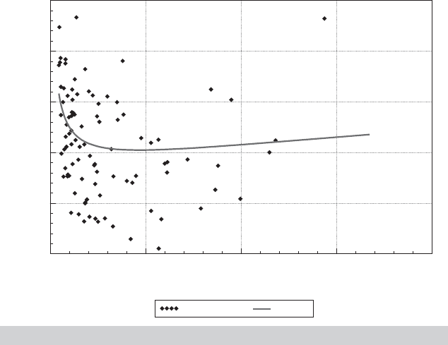
FIGURE 10.1

Predicted and Actual Average Costs.

things to note are the dramatically smaller standard errors and the now positive (and

reasonable) estimate of the capital coefﬁcient. The estimates of economies of scale in

the basic Cobb–Douglas model are 1/β

= 1.39 (column 1) and 1.31 (column 3), which

suggest some increasing returns to scale. Nerlove, however, had found evidence that at

extremely large ﬁrm sizes, economies of scale diminished and eventually disappeared.

To account for this (essentially a classical U-shaped average cost curve), he appended a

quadratic term in log output in the cost function. The single equation and multivariate

regression estimates are given in the second and fourth sets of results.

The quadratic output term gives the cost function the expected U-shape. We can

determine the point where average cost reaches its minimum by equating ∂ ln C/∂ ln Q

to 1. This is Q

∗

= exp[(1 − β

)/(2β

)]. For the multivariate regression, this value is

∗

= 4665. About 85 percent of the ﬁrms in the sample had output less than this, so by

these estimates, most ﬁrms in the sample had not yet exhausted the available economies

of scale. Figure 10.1 shows predicted and actual average costs for the sample. (To obtain

a reasonable scale, the smallest one third of the ﬁrms are omitted from the ﬁgure.)

Predicted average costs are computed at the sample averages of the input prices. The

ﬁgure does reveal that that beyond a quite small scale, the economies of scale, while

perhaps statistically signiﬁcant, are economically quite small.

10.5.2 FLEXIBLE FUNCTIONAL FORMS: THE TRANSLOG

COST FUNCTION

The literatures on production and cost and on utility and demand have evolved in

several directions. In the area of models of producer behavior, the classic paper by

Arrow et al. (1961) called into question the inherent restriction of the Cobb–Douglas

CHAPTER 10

✦

Systems of Equations

311

model that all elasticities of factor substitution are equal to 1. Researchers have since

developed numerous ﬂexible functions that allow substitution to be unrestricted (i.e.,

not even constant).

Similar strands of literature have appeared in the analysis of

commodity demands.

In this section, we examine in detail a model of production.

Suppose that production is characterized by a production function, Q = f (x).

The solution to the problem of minimizing the cost of producing a speciﬁed output

rate given a set of factor prices produces the cost-minimizing set of factor demands

= x

(Q, p). The total cost of production is given by the cost function,

C =



i=1

(Q, p) = C(Q, p). (10-31)

If there are constant returns to scale, then it can be shown that C = Qc(p) or

C/Q = c(p),

where c(p) is the unit or average cost function.

The cost-minimizing factor demands

are obtained by applying Shephard’s (1970) lemma, which states that if C(Q, p) gives

the minimum total cost of production, then the cost-minimizing set of factor demands

is given by

∗

∂C(Q, p)

∂p

Q∂c(p)

∂p

. (10-32)

Alternatively, by differentiating logarithmically, we obtain the cost-minimizing factor

cost shares:

∂ ln C(Q, p)

∂ ln p

. (10-33)

With constant returns to scale, ln C(Q, p) = ln Q + ln c(p),so

∂ ln c(p)

∂ ln p

. (10-34)

In many empirical studies, the objects of estimation are the elasticities of factor substi-

tution and the own price elasticities of demand, which are given by

c(∂

c/∂ p

∂p

)

(∂c/∂ p

)(∂c/∂ p

)

and

= s

See, in particular, Berndt and Christensen (1973). Two useful surveys of the topic are Jorgenson (1983) and

Diewert (1974).

See, for example, Christensen, Jorgenson, and Lau (1975) and two surveys, Deaton and Muellbauer (1980)

and Deaton (1983). Berndt (1990) contains many useful results.

The Cobb–Douglas function of the previous section gives an illustration. The restriction of constant returns

to scale is β

=1, which is equivalent to C = Qc(p). Nerlove’s more general version of the cost function

allows nonconstant returns to scale. See Christensen and Greene (1976) and Diewert (1974) for some of the

formalities of the cost function and its relationship to the structure of production.

312

PART II

✦

Generalized Regression Model and Equation Systems

By suitably parameterizing the cost function (10-31) and the cost shares (10-34), we

obtain an M or M +1 equation econometric model that can be used to estimate these

quantities.

The transcendental logarithmic or translog function is the most frequently used

ﬂexible function in empirical work.

By expanding ln c(p) in a second-order Taylor

series about the point ln p = 0, we obtain

ln c ≈ β



i=1



∂ ln c

∂ ln p



log p



i=1



j=1



∂

ln c

∂ ln p



ln p

, (10-35)

where all derivatives are evaluated at the expansion point. If we treat these derivatives

as the coefﬁcients, then the cost function becomes

ln c = β

+ β

ln p

+···+β

ln p

+ δ





+ δ

ln p

+δ





+···+δ





. (10-36)

This is the translog cost function. If δ

equals zero, then it reduces to the Cobb–Douglas

function we looked at earlier. The cost shares are given by

∂ ln c

∂ ln p

= β

+ δ

ln p

+ δ

ln p

+···+δ

ln p

∂ ln c

∂ ln p

= β

+ δ

ln p

+ δ

ln p

+···+δ

ln p

∂ ln c

∂ ln p

= β

+ δ

ln p

+ δ

ln p

+···+δ

ln p

(10-37)

The cost shares must sum to 1, which requires,

+ β

+···+β

= 1,



i=1

= 0 (column sums equal zero), (10-38)



j=1

= 0 (row sums equal zero).

We will also impose the (theoretical) symmetry restriction, δ

= δ

The system of share equations provides a seemingly unrelated regressions model

that can be used to estimate the parameters of the model.

To make the model

The cost function is only one of several approaches to this study. See Jorgenson (1983) for a discussion.

See Example 2.4. The function was developed by Kmenta (1967) as a means of approximating the CES

production function and was introduced formally in a series of papers by Berndt, Christensen, Jorgenson,

and Lau, including Berndt and Christensen (1973) and Christensen et al. (1975). The literature has produced

something of a competition in the development of exotic functional forms. The translog function has remained

the most popular, however, and by one account, Guilkey, Lovell, and Sickles (1983) is the most reliable of

several available alternatives. See also Example 5.4.

The cost function may be included, if desired, which will provide an estimate of β

but is otherwise inessential.

Absent the assumption of constant returns to scale, however, the cost function will contain parameters of

interest that do not appear in the share equations. As such, one would want to include it in the model. See

Christensen and Greene (1976) for an application.

CHAPTER 10

✦

Systems of Equations

313

TABLE 10.3

Parameter Estimates (standard errors in parentheses)

0.05682 (0.00131) δ

−0.02169

∗

(0.00963)

0.25355 (0.001987) δ

0.07488 (0.00639)

0.04383 (0.00105) δ

−0.00321 (0.00275)

0.64580

∗

(0.00299) δ

−0.07169

∗

(0.00941)

0.02987 (0.00575) δ

0.02938 (0.00741)

0.0000221 (0.00367) δ

−0.01797

∗

(0.01075)

−0.00820 (0.00406) δ

0.11134

∗

(0.02239)

∗

Estimated indirectly using (10-38).

operational, we must impose the restrictions in (10-38) and solve the problem of singu-

larity of the disturbance covariance matrix of the share equations. The ﬁrst is accom-

plished by dividing the ﬁrst M −1 prices by the Mth, thus eliminating the last term in

each row and column of the parameter matrix. As in the Cobb–Douglas model, we

obtain a nonsingular system by dropping the Mth share equation. We compute max-

imum likelihood estimates of the parameters to ensure invariance with respect to the

choice of which share equation we drop. For the translog cost function, the elastici-

ties of substitution are particularly simple to compute once the parameters have been

estimated:

+ s

,θ

+ s

− 1)

. (10-39)

These elasticities will differ at every data point. It is common to compute them at some

central point such as the means of the data.

Example 10.3 A Cost Function for U.S. Manufacturing

A number of recent studies using the translog methodology have used a four-factor model,

with capital K , labor L, energy E, and materials M, the factors of production. Among the ﬁrst

studies to employ this methodology was Berndt and Wood’s (1975) estimation of a translog

cost function for the U.S. manufacturing sector. The three factor shares used to estimate the

model are

= β

+ δ





+ δ





+ δ





= β

+ δ





+ δ





+ δ





= β

+ δ





+ δ





+ δ





Berndt and Wood’s data are reproduced in Appendix Table F10.2. Constrained FGLS esti-

mates of the parameters presented in Table 10.3 were obtained by constructing the “pooled

They will also be highly nonlinear functions of the parameters and the data. A method of computing asymp-

totic standard errors for the estimated elasticities is presented in Anderson and Thursby (1986). Krinsky and

Robb (1986, 1990) (see Section 15.3) proposed their method as an alternative approach to this computation.

314

PART II

✦

Generalized Regression Model and Equation Systems

TABLE 10.4

Estimated Elasticities

Capital Labor Energy Materials

Cost Shares for 1959

Fitted shares 0.05646 0.27454 0.04424 0.62476

Actual shares 0.06185 0.27303 0.04563 0.61948

Implied Elasticities of Substitution, 1959

Capital −7.34124

Labor 1.0014 −1.64902

Energy −2.28422 0.73556 −6.59124

Materials 0.38512 0.58205 0.34994 −0.31536

Implied Own Price Elasticities

−0.41448 −0.45274 −0.29161 −0.19702

regression” in (10-19) with data matrices

y =





(10-40)

X =



i 00lnP

ln P

000

0i0 0 lnP

0lnP

ln P

00 i 0 0 lnP

0lnP

ln P





= (β

, β

, δ

Estimates are then obtained using the two-step procedure in (10-7) and (10-9).

The full set

of estimates are given in Table 10.4. The parameters not estimated directly in (10-36) are

computed using (10-38).

The implied estimates of the elasticities of substitution and demand for 1959 (the central

year in the data) are derived in Table 10.4 using the ﬁtted cost shares and the estimated

parameters in (10-39). The departure from the Cobb–Douglas model with unit elasticities is

substantial. For example, the results suggest almost no substitutability between energy and

labor and some complementarity between capital and energy.

10.6 SIMULTANEOUS EQUATIONS MODELS

There is a qualitative difference between the market equilibrium model suggested in

the chapter Introduction,

Demand

= α

+ α

Price + α

Income + d



α + ε

Demand

Supply

= β

+ β

Price + s



β + ε

Supply

Equilibrium

= Q

Demand

= Q

Supply

These estimates do not match those reported by Berndt and Wood. They used an iterative estimator, whereas

ours is two step FGLS. To purge their data of possible correlation with the disturbances, they ﬁrst regressed

the prices on 10 exogenous macroeconomic variables, such as U.S. population, government purchases of labor

services, real exports of durable goods and U.S. tangible capital stock, and then based their analysis on the

ﬁtted values. The estimates given here are, in general quite close to those given by Berndt and Wood. For

example, their estimates of the ﬁrst ﬁve parameters are 0.0564, 0.2539, 0.0442, 0.6455, and 0.0254.

Berndt and Wood’s estimate of θ

for 1959 is 0.64.

CHAPTER 10

✦

Systems of Equations

315

and the other examples considered thus far. The seemingly unrelated regression model,

= x



+ ε

derives from a set of regression equations that are connected through the disturbances.

The regressors, x

are exogenous and vary autonomously for reasons that are not

explained within the model. Thus, the coefﬁcients are directly interpretable as partial ef-

fects and can be estimated by least squares or other methods that are based on the condi-

tional mean functions, E[y

] = x



β. In a model such as the preceding equilibrium

model, the relationships are explicit and neither of the two market equations is a regres-

sion model. As a consequence, the partial equilibrium experiment of changing the price

and inducing a change in the equilibrium quantity so as to elicit an estimate of the price

elasticity of demand, α

(or supply elasticity, β

) makes no sense. The model is of the

joint determination of quantity and price. Price changes when the market equilibrium

changes, but that is induced by changes in other factors, such as changes in incomes or

other variables that affect the supply function. (See Figure 8.1 for a graphical treatment.)

As we saw in Example 8.4, least squares regression of observed equilibrium quanti-

ties on price and the other factors will compute an ambiguous mixture of the supply and

demand functions. The result follows from the endogeneity of Price in either equation.

“Simultaneous equations models” arise in settings such as this one, in which the set of

equations are interdependent by design. Simultaneous equations models will ﬁt in the

framework developed in Chapter 8, where we considered equations in which some of

the right-hand-side variables are endogenous—that is, correlated with the disturbances.

The substantive difference at this point is the source of the endogeneity. In our treat-

ments in Chapter 8, endogeneity arose, for example, in the models of omitted variables,

measurement error, or endogenous treatment effects, essentially as an unintended de-

viation from the assumptions of the linear regression model. In the simultaneous equa-

tions framework, endogeneity is a fundamental part of the speciﬁcation. This section

will consider the issues of speciﬁcation and estimation in systems of simultaneous equa-

tions. We begin in Section 10.6.1 with a development of a general framework for the

analysis and a statement of some fundamental issues. Section 10.6.2 presents the simul-

taneous equations model as an extension of the seemingly unrelated regressions model

in Section 10.2. The ultimate objective of the analysis will be to learn about the model

coefﬁcients. The issue of whether this is even possible is considered in Section 10.6.3,

where we develop the issue of identiﬁcation. Once the identiﬁcation question is settled,

methods of estimation and inference are presented in Section 10.6.4 and 10.6.5.

10.6.1 SYSTEMS OF EQUATIONS

Consider a simpliﬁed version of the preceding equilibrium model, above,

demand equation: q

d,t

= α

+ α

+ ε

d,t

supply equation: q

s,t

= β

+ ε

s,t

equilibrium condition: q

d,t

= q

s,t

= q

These equations are structural equations in that they are derived from theory and each

purports to describe a particular aspect of the economy.

Because the model is one

The distinction between structural and nonstructural models is sometimes drawn on this basis. See, for

example, Cooley and LeRoy (1985).

316

PART II

✦

Generalized Regression Model and Equation Systems

of the joint determination of price and quantity, they are labeled jointly dependent or

endogenous variables. Income, x, is assumed to be determined outside of the model,

which makes it exogenous. The disturbances are added to the usual textbook description

to obtain an econometric model. All three equations are needed to determine the

equilibrium price and quantity, so the system is interdependent. Finally, because an

equilibrium solution for price and quantity in terms of income and the disturbances

is, indeed, implied (unless α

equals β

), the system is said to be a complete system of

equations. The completeness of the system requires that the number of equations equal

the number of endogenous variables. As a general rule, it is not possible to estimate all

the parameters of incomplete systems (although it may be possible to estimate some of

them).

Suppose that interest centers on estimating the demand elasticity α

. For simplicity,

assume that ε

and ε

are well behaved, classical disturbances with

E [ε

d,t

] = E [ε

s,t

] = 0,



d,t



= σ



s,t



= σ

E [ε

d,t

s,t

] = 0.

All variables are mutually uncorrelated with observations at different time periods.

Price, quantity, and income are measured in logarithms in deviations from their sample

means. Solving the equations for p and q in terms of x, ε

, and ε

produces the reduced

form of the model

p =

− α

− ε

− α

= π

x + v

q =

− α

= π

x + v

(10-41)

(Note the role of the “completeness” requirement that α

not equal β

It follows that Cov[ p,ε

] = σ

/(β

−α

) and Cov[p,ε

] =−σ

/(β

−α

) so neither

the demand nor the supply equation satisﬁes the assumptions of the classical regression

model. The price elasticity of demand cannot be consistently estimated by least squares

regression of q on x and p. This result is characteristic of simultaneous-equations models.

Because the endogenous variables are all correlated with the disturbances, the least

squares estimators of the parameters of equations with endogenous variables on the

right-hand side are inconsistent.

Suppose that we have a sample of T observations on p, q, and x such that

plim(1 / T )x



x = σ

Since least squares is inconsistent, we might instead use an instrumental variable es-

timator.

The only variable in the system that is not correlated with the disturbances

This failure of least squares is sometimes labeled simultaneous equations bias.

See Section 8.3.

CHAPTER 10

✦

Systems of Equations

317

is x. Consider, then, the IV estimator,

= q



x/p



x. This estimator has

plim

= plim



x / T



x / T

/(β

− α

)

/(β

− α

)

= β

Evidently, the parameter of the supply curve can be estimated by using an instrumental

variable estimator. In the least squares regression of p on x, the predicted values are

p = (p



x / x



x)x. It follows that in the instrumental variable regression the instrument is

p. That is,



Because



p =



is also the slope in a regression of q on these predicted values.

This interpretation deﬁnes the two-stage least squares estimator.

It would be desirable to use a similar device to estimate the parameters of the de-

mand equation, but unfortunately, we have exhausted the information in the sample. Not

only does least squares fail to estimate the demand equation, but without some further

assumptions, the sample contains no other information that can be used. This example

illustrates the problem of identiﬁcation alluded to in the introduction to this section.

The distinction between “exogenous” and “endogenous” variables in a model is a

subtle and sometimes controversial complication. It is the subject of a long literature.

We have drawn the distinction in a useful economic fashion at a few points in terms of

whether a variable in the model could reasonably be expected to vary “autonomously,”

independently of the other variables in the model. Thus, in a model of supply and de-

mand, the weather variable in a supply equation seems obviously to be exogenous in a

pure sense to the determination of price and quantity, whereas the current price clearly

is “endogenous” by any reasonable construction. Unfortunately, this neat classiﬁcation

is of fairly limited use in macroeconomics, where almost no variable can be said to be

truly exogenous in the fashion that most observers would understand the term. To take

a common example, the estimation of consumption functions by ordinary least squares,

as we did in some earlier examples, is usually treated as a respectable enterprise, even

though most macroeconomic models (including the examples given here) depart from a

consumption function in which income is exogenous. This departure has led analysts, for

better or worse, to draw the distinction largely on statistical grounds. The methodolog-

ical development in the literature has produced some consensus on this subject. As we

shall see, the deﬁnitions formalize the economic characterization we drew earlier. We

will loosely sketch a few results here for purposes of our derivations to follow. The inter-

ested reader is referred to the literature (and forewarned of some challenging reading).

Engle, Hendry, and Richard (1983) deﬁne a set of variables x

in a parameterized

model to be weakly exogenous if the full model can be written in terms of a marginal

probability distribution for x

and a conditional distribution for y

such that estimation

of the parameters of the conditional distribution is no less efﬁcient than estimation of

the full set of parameters of the joint distribution. This case will be true if none of the

parameters in the conditional distribution appears in the marginal distribution for x

In the present context, we will need this sort of construction to derive reduced forms

the way we did previously. With reference to time-series applications (although the

notion extends to cross sections as well), variables x

are said to be predetermined in

the model if x

is independent of all subsequent structural disturbances ε

t+s

for s ≥ 0.

318

PART II

✦

Generalized Regression Model and Equation Systems

Variables that are predetermined in a model can be treated, at least asymptotically, as

if they were exogenous in the sense that consistent estimators can be derived when

they appear as regressors. We will use this result in Chapter 21, when we derive the

properties of regressions containing lagged values of the dependent variable. A related

concept is Granger (1969)–Sims (1977) causality. Granger causality (a kind of statistical

feedback) is absent when f (x

t−1

, y

t−1

) equals f (x

t−1

). The deﬁnition states that

in the conditional distribution, lagged values of y

add no information to explanation

of movements of x

beyond that provided by lagged values of x

itself. This concept is

useful in the construction of forecasting models. Finally, if x

is weakly exogenous and

if y

t−1

does not Granger cause x

, then x

is strongly exogenous.

10.6.2 A GENERAL NOTATION FOR LINEAR SIMULTANEOUS

EQUATIONS MODELS

The structural form of the model is

+ γ

+···+γ

+ β

+···+β

= ε

+ γ

+···+γ

+ β

+···+β

= ε

(10-42)

+ γ

+···+γ

+ β

+···+β

= ε

There are M equations and M endogenous variables, denoted y

,...,y

. There are K

exogenous variables, x

,...,x

, that may include predetermined values of y

,...,y

as well. The ﬁrst element of x

will usually be the constant, 1. Finally, ε

,...,ε

are the

structural disturbances. The subscript t will be used to index observations, t = 1,...,T.

In matrix terms, the system may be written

··· y

]

⎡

⎢

⎣

··· γ

⎤

⎥

⎦

+[x

··· x

]

⎡

⎢

⎣

··· β

⎤

⎥

⎦

= [

··· ε

]

We will be restricting our attention to linear models. Nonlinear systems occupy another strand of literature

in this area. Nonlinear systems bring forth numerous complications beyond those discussed here and are

beyond the scope of this text. Gallant (1987), Gallant and Holly (1980), Gallant and White (1988), Davidson

and MacKinnon (2004), and Wooldridge (2002a) provide further discussion.

For the present, it is convenient to ignore the special nature of lagged endogenous variables and treat them

the same as the strictly exogenous variables.