Greene W.H. Econometric Analysis
Подождите немного. Документ загружается.

CHAPTER 14
✦
Maximum Likelihood Estimation
559
The information matrix for this log-likelihood is
−E
⎡
⎢
⎢
⎢
⎢
⎢
⎢
⎣
∂
2
ln L
∂
⎛
⎝
β
σ
2
u
ρ
⎞
⎠
∂
β
σ
2
u
ρ
⎤
⎥
⎥
⎥
⎥
⎥
⎥
⎦
=
⎡
⎢
⎢
⎢
⎢
⎢
⎢
⎢
⎣
1
σ
2
u
X
−1
X0 0
0
T
2σ
4
u
ρ
σ
2
u
(1 − ρ
2
)
0
ρ
σ
2
u
(1 − ρ
2
)
T − 2
1 − ρ
2
+
1 + ρ
2
(1 − ρ
2
)
2
⎤
⎥
⎥
⎥
⎥
⎥
⎥
⎥
⎦
.
(14-64)
Note that the diagonal elements in the matrix are O(T). But the (2, 3) and (3, 2)
elements are constants of O(1) that will, like the second part of the (3, 3) element,
become minimal as T increases. Dropping these “end effects” (and treating T − 2as
the same as T when T increases) produces a diagonal matrix from which we extract the
standard approximations for the MLEs in this model:
Asy. Var[
ˆ
β] = σ
2
u
(X
−1
X)
−1
,
Asy. Var
ˆσ
2
u
=
2σ
4
u
T
, (14-65)
Asy. Var[ ˆρ] =
1 − ρ
2
T
.
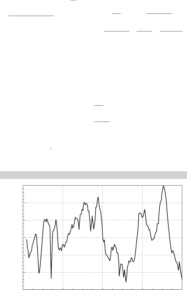
Example 14.7 Autocorrelation in a Money Demand Equation
Using the macroeconomic data in Table F5.2, we fit a money demand equation,
ln( M1/CPI
u)
t
= β
1
+ β
2
ln Real GDP
t
+ β
3
ln T-bill rate
t
+ ε
t
.
The least squares residuals shown in Figure 14.3 display the typical pattern for a highly
autocorrelated series.
FIGURE 14.3
Residuals from Estimated Money Demand Equation.
0.150
1949 1962 1975
Quarter
1988 2001
0.100
0.050
0.000
0.050
0.100
0.150
Residual

560
PART III
✦
Estimation Methodology
TABLE 14.4
Estimates of Money Demand Equation:
T = 204
OLS Prais and Winsten Maximum Likelihood
Variable Estimate Std. Error Estimate Std. Error Estimate Std. Error
Constant −2.1316 0.09100 −1.4755 0.2550 −1.6319 0.4296
Ln real GDP 0.3519 0.01205 0.2549 0.03097 0.2731 0.0518
Ln T-bill rate −0.1249 0.009841 −0.02666 0.007007 −0.02522 0.006941
σ
ε
0.06185 0.07767 0.07571
σ
u
0.06185 0.01298 0.01273
ρ 0. 0. 0.9557 0.02061 0.9858 0.01180
The simple first-order autocorrelation of the ordinary least squares residuals is r = 1 −
d/2 = 0.9557, where d is the Durbin–Watson Statistic in (20-23). We then refit the model
using the Prais and Winsten FGLS estimator and the maximum likelihood estimator using
the Beach and MacKinnon algorithm. The results are shown in Table 14.4. Although the OLS
estimator is consistent in this model, nonetheless, the FGLS and ML estimates are quite
different.
14.9.3 SEEMINGLY UNRELATED REGRESSION MODELS
The general form of the seemingly unrelated regression (SUR) model is given in
(10-1)–(10-3);
y
i
= X
i
β
i
+ ε
i
, i = 1,...,M,
E[ε
i
|X
1
,...,X
M
] = 0, (14-66)
E[ε
i
ε
j
|X
1
,...,X
M
] = σ
ij
I.
FGLS estimation of this model is examined in detail in Section 10.2.3. We will now
add the assumption of normally distributed disturbances to the model and develop the
maximum likelihood estimators. Given the covariance structure defined in (14-66), the
joint normality assumption applies to the vector of M disturbances observed at time t,
which we write as
ε
t
|X
1
,...,X
M
∼ N[0, ], t = 1,...,T. (14-67)
14.9.3.a The Pooled Model
The pooled model, in which all coefficient vectors are equal, provides a convenient
starting point. With the assumption of equal coefficient vectors, the regression model
becomes
y
it
= x
it
β + ε
it
,
E[ε
it
|X
1
,...,X
M
] = 0, (14-68)
E[ε
it
ε
js
|X
1
,...,X
M
] = σ
ij
if t = s, and0ift = s.
This is a model of heteroscedasticity and cross-sectional correlation. With multivariate
normality, the log-likelihood is
ln L =
T
t=1
−
M
2
ln 2π −
1
2
ln ||−
1
2
ε
t
−1
ε
t
. (14-69)

CHAPTER 14
✦
Maximum Likelihood Estimation
561
As we saw earlier, the efficient estimator for this model is GLS as shown in (10-21).
Because the elements of must be estimated, the FGLS estimator based on (10-9) is
used.
As we have seen in several applications now, the maximum likelihood estimator of
β, given , is GLS, based on (10-21). The maximum likelihood estimator of is
ˆσ
ij
=
y
i
− X
i
ˆ
ˆ
β
ML
y
j
− X
j
ˆ
ˆ
β
ML
T
=
ˆε
i
ˆε
j
T
(14-70)
based on the MLE of β. If each MLE requires the other, how can we proceed to obtain
both? The answer is provided by Oberhofer and Kmenta (1974), who show that for
certain models, including this one, one can iterate back and forth between the two esti-
mators. Thus, the MLEs are obtained by iterating to convergence between (14-70) and
ˆ
ˆ
β = [X
ˆ
−1
X]
−1
[X
ˆ
−1
y]. (14-71)
The process may begin with the (consistent) ordinary least squares estimator, then
(14-70), and so on. The computations are simple, using basic matrix algebra. Hypothe-
sis tests about β may be done using the familiar Wald statistic. The appropriate estimator
of the asymptotic covariance matrix is the inverse matrix in brackets in (10-21).
For testing the hypothesis that the off-diagonal elements of are zero—that is, that
there is no correlation across firms—there are three approaches. The likelihood ratio
test is based on the statistic
λ
LR
= T(ln |
ˆ
heteroscedastic
|−ln |
ˆ
general
|) = T
M
i=1
ln ˆσ
2
i
− ln |
ˆ
|
, (14-72)
where ˆσ
2
i
are the estimates of σ
2
i
obtained from the maximum likelihood estimates
of the groupwise heteroscedastic model and
ˆ
is the maximum likelihood estimator
in the unrestricted model. (Note how the excess variation produced by the restrictive
model is used to construct the test.) The large-sample distribution of the statistic is chi-
squared with M(M −1)/2 degrees of freedom. The Lagrange multiplier test developed
by Breusch and Pagan (1980) provides an alternative. The general form of the statistic is
λ
LM
= T
n
i=2
i−1
j=1
r
2
ij
, (14-73)
where r
2
ij
is the ijth residual correlation coefficient. If every equation had a different
parameter vector, then equation specific ordinary least squares would be efficient (and
ML) and we would compute r
ij
from the OLS residuals (assuming that there are suffi-
cient observations for the computation). Here, however, we are assuming only a single-
parameter vector. Therefore, the appropriate basis for computing the correlations is the
residuals from the iterated estimator in the groupwise heteroscedastic model, that is,
the same residuals used to compute ˆσ
2
i
. (An asymptotically valid approximation to the
test can be based on the FGLS residuals instead.) Note that this is not a procedure for
testing all the way down to the classical, homoscedastic regression model. That case in-
volves different LM and LR statistics based on the groupwise heteroscedasticity model.
If either the LR statistic in (14-72) or the LM statistic in (14-73) are smaller than the
critical value from the table, the conclusion, based on this test, is that the appropriate
model is the groupwise heteroscedastic model.

562
PART III
✦
Estimation Methodology
14.9.3.b The SUR Model
The Oberhofer–Kmenta (1974) conditions are met for the seemingly unrelated regres-
sions model, so maximum likelihood estimates can be obtained by iterating the FGLS
procedure. We note, once again, that this procedure presumes the use of (10-9) for esti-
mation of σ
ij
at each iteration. Maximum likelihood enjoys no advantages over FGLS
in its asymptotic properties.
20
Whether it would be preferable in a small sample is an
open question whose answer will depend on the particular data set.
14.9.3.c Exclusion Restrictions
By simply inserting the special form of in the log-likelihood function for the gen-
eralized regression model in (14-48), we can consider direct maximization instead of
iterated FGLS. It is useful, however, to reexamine the model in a somewhat different
formulation. This alternative construction of the likelihood function appears in many
other related models in a number of literatures.
Consider one observation on each of the M dependent variables and their associated
regressors. We wish to arrange this observation horizontally instead of vertically. The
model for this observation can be written
[y
1
y
2
··· y
M
]
t
= [x
∗
t
]
[π
1
π
2
··· π
M
] + [ε
1
ε
2
··· ε
M
]
t
= [x
∗
t
]
+ E,
(14-74)
where x
∗
t
is the full set of all K
∗
different independent variables that appear in the model.
The parameter matrix then has one column for each equation, but the columns are not
the same as β
i
in (14-66) unless every variable happens to appear in every equation.
Otherwise, in the ith equation, π
i
will have a number of zeros in it, each one imposing
an exclusion restriction. For example, consider a two-equation model for production
costs for two airlines,
C
1t
= α
1
+ β
1P
P
1t
+ β
1L
LF
1t
+ ε
1t
,
C
2t
= α
2
+ β
2P
P
2t
+ β
2L
LF
2t
+ ε
2t
,
where C is cost, P is fuel price, and LF is load factor. The tth observation would be
[C
1
C
2
]
t
= [1 P
1
LF
1
P
2
LF
2
]
t
⎡
⎢
⎢
⎢
⎢
⎢
⎢
⎣
α
1
α
2
β
1P
0
β
1L
0
0 β
2P
0 β
2L
⎤
⎥
⎥
⎥
⎥
⎥
⎥
⎦
+ [ε
1
ε
2
]
t
.
This vector is one observation. Let ε
t
be the vector of M disturbances for this
observation arranged, for now, in a column. Then E [ε
t
ε
t
] = . The log of the joint
normal density of these M disturbances is
ln L
t
=−
M
2
ln(2π) −
1
2
ln||−
1
2
ε
t
−1
ε
t
. (14-75)
20
Jensen (1995) considers some variation on the computation of the asymptotic covariance matrix for the
estimator that allows for the possibility that the normality assumption might be violated.

CHAPTER 14
✦
Maximum Likelihood Estimation
563
The log-likelihood for a sample of T joint observations is the sum of these over t:
ln L =
T
t=1
ln L
t
=−
MT
2
ln(2π) −
T
2
ln||−
1
2
T
t=1
ε
t
−1
ε
t
. (14-76)
The term in the summation in (14-76) is a scalar that equals its trace. We can always
permute the matrices in a trace, so
T
t=1
ε
t
−1
ε
t
=
T
t=1
tr
ε
t
−1
ε
t
=
T
t=1
tr
−1
ε
t
ε
t
. (14-77)
This can be further simplified. The sum of the traces of T matrices equals the trace of
the sum of the matrices [see (A-91)]. We will now also be able to move the constant
matrix,
−1
, outside the summation. Finally, it will prove useful to multiply and divide
by T. Combining all three steps, we obtain
T
t=1
tr
−1
ε
t
ε
t
= T tr
−1
1
T
T
t=1
ε
t
ε
t
= T tr(
−1
W), (14-78)
where
W
ij
=
1
T
T
t=1
ε
ti
ε
tj
.
Because this step uses actual disturbances, E [W
ij
] = σ
ij
; W is the M × M matrix we
would use to estimate if the ε’s were actually observed. Inserting this result in the
log-likelihood, we have
ln L =−
T
2
[M ln(2π) + ln||+tr(
−1
W)]. (14-79)
We now consider maximizing this function.
It has been shown
21
that
∂ ln L
∂
=
T
2
X
∗
E
−1
,
∂ ln L
∂
=−
T
2
−1
( − W)
−1
,
(14-80)
where the x
∗
t
in (14-74) is row t of X
∗
. Equating the second of these derivatives to a zero
matrix, we see that given the maximum likelihood estimates of the slope parameters, the
maximum likelihood estimator of is W, the matrix of mean residual sums of squares
and cross products—that is, the matrix we have used for FGLS. [Notice that there is no
correction for degrees of freedom; ∂ ln L/∂ = 0 implies (10-9).]
We also know that because this model is a generalized regression model, the maxi-
mum likelihood estimator of the parameter matrix [β] must be equivalent to the FGLS
estimator we discussed earlier.
22
It is useful to go a step further. If we insert our solution
21
See, for example, Joreskog (1973).
22
This equivalence establishes the Oberhofer–Kmenta conditions.

564
PART III
✦
Estimation Methodology
for in the likelihood function, then we obtain the concentrated log-likelihood,
ln L
c
=−
T
2
[M(1 + ln(2π)) + ln|W|]. (14-81)
We have shown, therefore, that the criterion for choosing the maximum likelihood
estimator of β is
ˆ
β
ML
= Min
β
1
2
ln|W|, (14-82)
subject to the exclusion restrictions. This important result reappears in many other mod-
els and settings. This minimization must be done subject to the constraints in the pa-
rameter matrix. In our two-equation example, there are two blocks of zeros in the
parameter matrix, which must be present in the MLE as well. The estimator of β is the
set of nonzero elements in the parameter matrix in (14-74).
The likelihood ratio statistic is an alternative to the F statistic discussed earlier for
testing hypotheses about β. The likelihood ratio statistic is
23
λ =−2(log L
r
− log L
u
) = T(log|
ˆ
W
r
|−log|
ˆ
W
u
|), (14-83)
where
ˆ
W
r
and
ˆ
W
u
are the residual sums of squares and cross-product matrices using
the constrained and unconstrained estimators, respectively. Under the null hypothesis
of the restrictions, the limiting distribution of the likelihood ratio statistic is chi-squared
with degrees of freedom equal to the number of restrictions. This procedure can also
be used to test the homogeneity restriction in the multivariate regression model. The
restricted model is the pooled model discussed in the preceding section.
It may also be of interest to test whether is a diagonal matrix. Two possible
approaches were suggested in Section 14.9.3a [see (14-72) and (14-73)]. The unrestricted
model is the one we are using here, whereas the restricted model is the groupwise
heteroscedastic model of Section 9.8.2 (Example 9.5), without the restriction of equal-
parameter vectors. As such, the restricted model reduces to separate regression models,
estimable by ordinary least squares. The likelihood ratio statistic would be
λ
LR
= T
M
i=1
log ˆσ
2
i
− log |
ˆ
|
, (14-84)
where ˆσ
2
i
is e
i
e
i
/T from the individual least squares regressions and
ˆ
is the maxi-
mum likelihood estimate of . This statistic has a limiting chi-squared distribution with
M(M − 1)/2 degrees of freedom under the hypothesis. The alternative suggested by
Breusch and Pagan (1980) is the Lagrange multiplier statistic,
λ
LM
= T
M
i=2
i−1
j=1
r
2
ij
, (14-85)
where r
ij
is the estimated correlation ˆσ
ij
/[ˆσ
ii
ˆσ
jj
]
1/2
. This statistic also has a limiting chi-
squared distribution with M(M −1)/2 degrees of freedom. This test has the advantage
that it does not require computation of the maximum likelihood estimator of , because
it is based on the OLS residuals.
23
See Attfield (1998) for refinements of this calculation to improve the small sample performance.

CHAPTER 14
✦
Maximum Likelihood Estimation
565
Example 14.8 ML Estimates of a Seemingly Unrelated
Regressions Model
Although a bit dated, the Grunfeld data used in Application 11.2 have withstood the test of
time and are still the standard data set used to demonstrate the SUR model. The data in
Appendix Table F10.4 are for 10 firms and 20 years (1935–1954). For the purpose of this
illustration, we will use the first four firms. [The data are downloaded from the Web site for
Baltagi (2005), at http://www.wiley.com/legacy/wileychi/baltagi/supp/Grunfeld.fil. See also
Kleiber and Zeileis (2010).]
The model is an investment equation:
I
it
= β
1i
+ β
2i
F
it
+ β
3i
C
it
+ ε
it
, t = 1, ..., 20, i = 1, ..., 10,
where
I
it
= real gross investment for firm i in year t,
F
it
= real value of the firm-shares outstanding,
C
it
= real value of the capital stock.
The OLS estimates for the four equations are shown in the left panel of Table 14.5. The
correlation matrix for the four OLS residual vectors is
R
e
=
⎡
⎢
⎣
1 −0.261 0.279 −0.273
−0.261 1 0.428 0.338
0.279 0.428 1 −0.0679
−0.273 0.338 −0.0679 1
⎤
⎥
⎦
.
Before turning to the FGLS and MLE estimates, we carry out the LM test against the null
hypothesis that the regressions are actually unrelated. We leave as an exercise to show that
the LM statistic in (14-85) can be computed as
λ
LM
= ( T/2)[trace( R
e
R
e
) − M] = 10.451.
The 95 percent critical value from the chi squared distribution with 6 degrees of freedom is
12.59, so at this point, it appears that the null hypothesis is not rejected. We will proceed in
spite of this finding.
TABLE 14.5
Estimated Investment Equations
OLS FGLS MLE
Firm Variable Estimate St. Err. Estimate St. Err. Estimate St. Err.
Constant −149.78 97.58 −160.68 90.41 −179.41 86.66
1
F 0.1192 0.02382 0.1205 0.02187 0.1248 0.02086
C 0.3714 0.03418 0.3800 0.03311 0.3802 0.03266
Constant −49.19 136.52 21.16 116.18 36.46 106.18
2
F 0.1749 0.06841 0.1304 0.05737 0.1244 0.05191
C 0.3896 0.1312 0.4485 0.1225 0.4367 0.1171
Constant −9.956 28.92 −19.72 26.58 −24.10 25.80
3
F 0.02655 0.01435 0.03464 0.01279 0.03808 0.01217
C 0.1517 0.02370 0.1368 0.02249 0.1311 0.02223
Constant −6.190 12.45 0.9366 11.59 2.581 11.54
4
F 0.07795 0.01841 0.06785 0.01705 0.06564 0.01698
C 0.3157 0.02656 0.3146 0.02606 0.3137 0.02617
566
PART III
✦
Estimation Methodology
The next step is to compute the covariance matrix for the OLS residuals using
W = (1/T )E
E =
⎡
⎢
⎣
7160.29 −1967.05 607.533 −282.756
−1967.05 7904.66 978.45 367.84
607.533 978.45 660.829 −21.3757
− 282.756 367.84 −21.3757 149.872
⎤
⎥
⎦
,
where E is the 20 × 4 matrix of OLS residuals. Stacking the data in the partitioned matrices
X =
⎡
⎢
⎣
X
1
000
0X
2
00
00X
3
0
000X
4
⎤
⎥
⎦
and y =
⎡
⎢
⎣
y
1
y
2
y
3
y
4
⎤
⎥
⎦
,
we now compute
ˆ
= W ⊗ I
20
and the FGLS estimates,
ˆ
β = [X
ˆ
−1
X]
−1
X
ˆ
−1
y.
The estimated asymptotic covariance matrix for the FGLS estimates is the bracketed inverse
matrix. These results are shown in the center panel in Table 14.5.
To compute the MLE, we will take advantage of the Oberhofer and Kmenta (1974) re-
sult and iterate the FGLS estimator. Using the FGLS coefficient vector, we recompute the
residuals, then recompute W, then reestimate β. The iteration is repeated until the estimated
parameter vector converges. We use as our convergence measure the following criterion
based on the change in the estimated parameter from iteration (s − 1) to iteration (s):
δ = [
ˆ
β(s) −
ˆ
β(s − 1)]
[X
[
ˆ
(s)]
−1
X][
ˆ
β(s) −
ˆ
β(s − 1)].
The sequence of values of this criterion function are: 0.21922, 0.16318, 0.00662, 0.00037,
0.00002367825, 0.000001563348, 0.1041980 × 10
−6
. We exit the iterations after iteration 7.
The ML estimates are shown in the right panel of Table 14.5.
We then carry out the likelihood ratio test of the null hypothesis of a diagonal covariance
matrix. The maximum likelihood estimate of is
ˆ
=
⎡
⎢
⎣
7235.46 −2455.13 615.167 −325.413
−2455.13 8146.41 1288.66 427.011
615.167 1288.66 702.268 2.51786
−325.413 427.011 2.51786 153.889
⎤
⎥
⎦
The estimate for the constrained model is the diagonal matrix formed from the diagonals of
W shown earlier for the OLS results. (The estimates are shown in boldface in the preceding
matrix.) The test statistic is then
LR = T (ln|diag(W) |−ln |
ˆ
|) = 18.55.
Recall that the critical value is 12.59. The results contradict the LM statistic. The hypothesis
of diagonal covariance matrix is now rejected.
Note that aside from the constants, the four sets of coefficient estimates are fairly similar.
Because of the constants, there seems little doubt that the pooling restriction will be rejected.
To find out, we compute the Wald statistic based on the MLE results. For testing
H
0
: β
1
= β
2
= β
3
= β
4
,
we can formulate the hypothesis as
H
0
: β
1
− β
4
= 0, β
2
− β
4
= 0, β
3
− β
4
= 0.
The Wald statistic is
λ
W
= (R
ˆ
β − q)
[RVR
]
−1
(R
ˆ
β − q) = 2190.96
CHAPTER 14
✦
Maximum Likelihood Estimation
567
where R =
I
3
00−I
3
0I
3
0 −I
3
00I
3
−I
3
, q =
0
0
0
, and V = [X
ˆ
−1
X]
−1
. Under the null hypothesis, the
Wald statistic has a limiting chi-squared distribution with 9 degrees of freedom. The critical
value is 16.92, so, as expected, the hypothesis is rejected. It may be that the difference is due
to the different constant terms. To test the hypothesis that the four pairs of slope coefficients
are equal, we replaced the I
3
in R with [0, I
2
], the 0s with 2 × 3 zero matrices and q with
a6× 1 zero vector, The resulting chi-squared statistic equals 229.005. The critical value is
12.59, so this hypothesis is rejected also.
14.9.4 SIMULTANEOUS EQUATIONS MODELS
In Chapter 10, we noted two approaches to maximum likelihood estimation in the
equation system
y
t
+ x
t
B = ε
t
,
(14-86)
ε
t
|X ∼ N[0,].
The limited information maximum likelihood (LIML) estimator is a single-equation
approach that estimates the parameters one equation at a time. The full information
maximum likelihood (FIML) estimator analyzes the full set of equations at one step.
Derivation of the LIML estimator is quite complicated. Lengthy treatments appear
in Anderson and Rubin (1948), Theil (1971), and Davidson and MacKinnon (1993,
Chapter 18). The mechanics of the computation are surprisingly simple, as shown earlier
(Section 10.6.4). The LIML estimates for Klein’s Model I appear in Example 10.6 with
the other single-equation and system estimators. For the practitioner, a useful result
is that the asymptotic variance of the two-stage least squares (2SLS) estimator, which
is yet simpler to compute, is the same as that of the LIML estimator. For practical
purposes, this would generally render the LIML estimator, with its additional normality
assumption, moot. The virtue of the LIML is largely theoretical—it provides a useful
benchmark for the analysis of the properties of single-equation estimators. The single
exception would be the invariance of the estimator to normalization of the equation
(i.e., which variable appears on the left of the equals sign). This turns out to be useful in
the context of analysis in the presence of weak instruments. (See Sections 8.7 and 10.6.6.)
The FIML estimator is much simpler to derive than the LIML estimator but con-
siderably more difficult to implement. To obtain the needed results, we first operated
on the reduced form
y
t
= x
t
+ v
t
,
(14-87)
v
t
|X ∼ N[0, ],
which is the seemingly unrelated regressions model analyzed at length in Chapter 10
and in Section 14.9.3. The complication is the restrictions imposed on the parameters,
=−B
−1
and = (
−1
)
(
−1
). (14-88)
As is now familiar from several applications, given estimates of and B in (14-86),
the estimator of is (1/T)E
E based on the residuals. We can even show fairly easily
that given and , the estimator of (−B) in (14-86) would be provided by the results
for the SUR model in Section 14.9.3.c (where we estimate the model subject to the
zero restrictions in the coefficient matrix). The complication in estimation is brought by

568
PART III
✦
Estimation Methodology
; this is a Jacobian. The term ln || appears in the log-likelihood function. Nonlinear
optimization over the nonzero elements in a function that includes this term is exceed-
ingly complicated. However, three-stage least squares (3SLS) has the same asymptotic
efficiency as the FIML estimator, again without the normality assumption and without
the practical complications.
The end result is that for the practitioner, the LIML and FIML estimators have
been supplanted in the literature by much simpler GMM estimators, 2SLS, H2SLS,
3SLS, and H3SLS. Interest remains in these estimators, but largely as a component of
the ongoing theoretical development.
14.9.5 MAXIMUM LIKELIHOOD ESTIMATION OF NONLINEAR
REGRESSION MODELS
In Chapter 7, we considered nonlinear regression models in which the nonlinearity in
the parameters appeared entirely on the right-hand side of the equation. Maximum
likelihood is used when the disturbances in a regression, or the dependent variable,
more generally, is not normally distributed. The geometric regression model provides
an application.
Example 14.9 Identification in a Loglinear Regression Model
In Example 7.6, we estimated an exponential regression model, of the form
E[Income|Age, Education, Female] = exp(γ
∗
1
+ γ
2
Age + γ
3
Education + γ
4
Female).
This loglinear conditional mean is consistent with several different distributions, including the
lognormal, Weibull, gamma, and exponential models. In each of these cases, the conditional
mean function is of the form
E[Income|x] = g(θ) exp(γ
1
+ x
γ
2
)
= exp(γ
∗
1
+ x
γ
2
),
where θ is an additional parameter of the distribution and γ
∗
1
= ln g(θ) +γ
1
. Two implications
are:
1. Nonlinear least squares (NLS) is robust at least to some failures of the distributional as-
sumption. The nonlinear least squares estimator of γ
2
will be consistent and asymptotically
normally distributed in all cases for which E[Income|x] = exp(γ
∗
1
+ x
γ
2
).
2. The NLS estimator cannot produce a consistent estimator of γ
1
; plimc
1
= γ
∗
1
, which varies
depending on the correct distribution. In the conditional mean function, any pair of values
for which γ
1
= ln g(θ ) + γ
1
is the same will lead to the same sum of squares. This is
a form of multicollinearity; the pseudoregressor for θ is ∂ E[Income|x]/∂θ = exp( γ
∗
1
+
x
γ
2
)[g
(θ ) /g(θ)] while that for γ
1
is ∂ E[Income|x]/∂γ
1
= exp(γ
∗
1
+ x
γ
2
). The first is a
constant multiple of the second.
NLS cannot provide separate estimates of θ and γ
1
while MLE can—see the example to
follow. Second, NLS might be less efficient than MLE since it does not use the information
about the distribution of the dependent variable. This second consideration is uncertain. For
estimation of γ
2
, the NLS estimator is less efficient for not using the distributional information.
However, that shortcoming might be offset because the NLS estimator does not attempt to
compute an independent estimator of the additional parameter, θ .
To illustrate, we reconsider the estimator in Example 7.6. The gamma regression model
specifies
f ( y|x) =
μ(x)
θ
( θ)
exp[−μ(x) y]y
θ−1
, y > 0, θ>0, μ( x) = exp(−γ
1
− x
γ
2
).