Greene W.H. Econometric Analysis

Подождите немного. Документ загружается.

CHAPTER 14

✦

Maximum Likelihood Estimation

569

TABLE 14.6

Estimated Gamma Regression Model

(2)

(1) Constrained (3) (4)

NLS NLS MLE NLS/MLE

Constant 1.22468 1.69331 3.36826 3.36380

(47722.5) (0.04408) (0.05048) (0.04408)

Age −0.00207 −0.00207 −0.00153 −0.00207

(0.00061) (0.00061) (0.00061) (0.00061)

Education −0.04792 −0.04792 −0.04975 −0.04792

(0.00247) (0.00247) (0.00286) (0.00247)

Female 0.00658 0.00658 0.00696 0.00658

(0.01373) (0.01373) (0.01322) (0.08677)

θ 0.62699 — 5.31474 5.31474

(29921.3) — (0.10894) (0.00000)

The conditional mean function for this model is

E[y|x] = θ/μ( x) = θ exp(γ

+ x



) = exp( γ

∗

+ x



Table 14.6 presents estimates of θ and (γ

, γ

). Estimated standard errors appear in parenthe-

ses. The estimates in columns (1), (2) and (4) are all computed using nonlinear least squares.

In (1), an attempt is made to estimate θ and γ

separately. The estimator “converged” on two

values. However, the estimated standard errors are essentially inﬁnite. The convergence to

anything at all is due to rounding error in the computer. The results in column (2) are for γ

∗

and

. The sums of squares for these two estimates as well as for those in (4) are all 112.19688,

indicating that the three results merely show three different sets of results for which γ

∗

is the

same. The full maximum likelihood estimates are presented in (3). Note that an estimate of

θ is obtained here because the assumed gamma distribution provides another independent

moment equation for this parameter, ∂ ln L/∂θ =−n ln ( θ) + 

(lny

− ln μ( x)) = 0, while

the normal equations for the sum of squares provides the same normal equation for θ and γ

The standard approach to modeling counts of events begins with the Poisson re-

gression model,

Prob[Y = y

] =

exp(−λ

)λ

,λ

= exp(x



β), y

= 0, 1,...

which has loglinear conditional mean function E[y

] = λ

. (The Poisson regression

model and other speciﬁcations for data on counts are discussed at length in Chapter 18.

We introduce the topic here to begin development of the MLE in a fairly straight-

forward, typical nonlinear setting.) Appendix Table F7.1 presents the Riphahn et al.

(2003) data, which we will use to analyze a count variable, DocVis, the number of visits

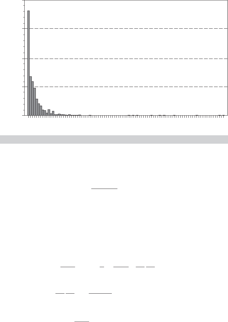
to physicans in the survey year. The histogram in Figure 14.4 shows a distinct spike at

zero followed by rapidly declining frequencies. While the Poisson distribution, which

is typically hump-shaped, can accommodate this conﬁguration if λ

is less than one,

the shape is nonetheless somewhat “non-Poisson.” [So-called Zero Inﬂation models

(discussed in Chapter 18) are often used for this situation.]

The geometric distribution,

f (y

) = θ

(1 − θ

)

,θ

= 1/(1 + λ

), λ

= exp(x



β), y

= 0, 1,...,

is a convenient speciﬁcation that produces the effect shown in Figure 14.4. (Note that,

formally, the speciﬁcation is used to model the number of failures before the ﬁrst success

570

PART III

✦

Estimation Methodology

0 5 10 15 20 25 30 35 40 45 50 55 60 65 70 75 80 85 90 95

DOCVIS

636

1272

1908

2544

Frequency

FIGURE 14.4

Histogram for Doctor Visits.

in successive independent trials each with success probability θ

, so in fact, it is misspec-

iﬁed as a model for counts. The model does provide a convenient and useful illustration,

however.) The conditional mean function is also E[y

] = λ

. The partial effects in

the model are

∂ E[y

]

∂x

= λ

β,

so this is a distinctly nonlinear regression model. We will construct a maximum likeli-

hood estimator, then compare the MLE to the nonlinear least squares and (misspeciﬁed)

linear least squares estimates.

The log-likelihood function is

ln L =



i=1

ln f (y

, β) =



i=1

ln θ

+ y

ln(1 − θ

The likelihood equations are

∂ ln L

∂β



i=1



−

1 − θ



dθ

dλ

∂λ

∂β

= 0.

Because

dθ

dλ

∂λ

∂β



−1

(1 + λ

)



=−θ

(1 − θ

the likelihood equations simplify to

∂ ln L

∂β



i=1

(θ

− (1 − θ

))x



i=1

(θ

(1 + y

) − 1)x

CHAPTER 14

✦

Maximum Likelihood Estimation

571

To estimate the asymptotic covariance matrix, we can use any of the three estimators

of Asy. Var [

MLE

]. The BHHH estimator would be

Est. Asy. Var

BHHH

[

MLE

] =





i=1



∂ ln f (y

β)

∂



∂ ln f (y

β)

∂







−1





i=1

(

(1 + y

) − 1)





The negative inverse of the second derivatives matrix evaluated at the MLE is



−

∂

ln L

∂

β∂





−1





i=1

(1 + y

)

(1 −





−1

Finally, as noted earlier, E[y

| x

] = λ

= (1 − θ

)/θ

, is known, so we can also use the

negative inverse of the expected second derivatives matrix,



−E



∂

ln L

∂

β∂





−1





i=1

(1 −





−1

To compute the estimates of the parameters, either Newton’s method,

t+1

−





−1

or the method of scoring,

t+1

−



]



−1

can be used, where H and g are the second and ﬁrst derivatives that will be evaluated

at the current estimates of the parameters. Like many models of this sort, there is a

convenient set of starting values, assuming the model contains a constant term. Because

E[y

] = λ

, if we start the slope parameters at zero, then a natural starting value for

the constant term is the log of ¯y.

Example 14.10 Geometric Regression Model for Doctor Visits

In Example 7.6, we considered nonlinear least squares estimation of a loglinear model for the

number of doctor visits variable shown in Figure 14.4. The data are drawn from the Riphahn

et al. (2003) data set in Appendix Table F7.1. We will continue that analysis here by ﬁtting a

more detailed model for the count variable DocVis. The conditional mean analyzed here is

ln E[DocVis

] = β

+ β

Age

+ β

Educ

+ β

Income

+ β

Kids

(This differs slightly from the model in Example 11.14. For this exercise, with an eye toward

the ﬁxed effects model in Example 14.13), we have speciﬁed a model that does not contain

any time-invariant variables, such as Female

.) Sample means for the variables in the model

are given in Table 14.7. Note, these data are a panel. In this exercise, we are ignoring that

fact, and ﬁtting a pooled model. We will turn to panel data treatments in the next section,

and revisit this application.

572

PART III

✦

Estimation Methodology

We used Newton’s method for the optimization, with starting values as suggested earlier.

The ﬁve iterations are as follows:

Variable Constant Age Educ Income Kids

Start values: 0.11580e+01 0.00000e+00 0.00000e+00 0.00000e+00 0.00000e+00

1st derivs. −0.25191e−08 −0.61777e+05 0.73202e+04 0.42575e+04 0.16464e+04

Parameters: 0.11580e+01 0.00000e+00 0.00000e+00 0.00000e+00 0.00000e+00

Iteration 1 F = 0.6287e+05 g



inv(H)g = 0.4367e+02

1st derivs. 0.48616e+03 −0.22449e+05 −0.57162e+04 −0.17112e+04 −0.16521e+03

Parameters: 0.11186e+01 0.17563e−01 −0.50263e−01 −0.46274e−01 −0.15609e+00

Iteration 2 F = 0.6192e+05 g



inv(H)g = 0.3547e+01

1st derivs. −0.31284e+01 −0.15595e+03 −0.37197e+02 −0.10630e+02 −0.77186e+00

Parameters: 0.10922e+01 0.17981e−01 −0.47303e−01 −0.46739e−01 −0.15683e+00

Iteration 3 F= 0.6192e+05 g



inv(H)g = 0.2598e−01

1st derivs. −0.18417e−03 −0.99368e−02 −0.21992e−02 −0.59354e−03 −0.25994e−04

Parameters: 0.10918e+01 0.17988e−01 −0.47274e−01 −0.46751e−01 −0.15686e+00

Iteration 4 F= 0.6192e+05 g



inv(H)g = 0.1831e−05

1st derivs. −0.35727e−11 0.86745e−10 −0.26302e−10 −0.61006e−11 −0.15620e−11

Parameters: 0.10918e+01 0.17988e−01 −0.47274e−01 −0.46751e−01 −0.15686e+00

Iteration 5 F= 0.6192e+05 g



inv(H)g = 0.1772e−12

Convergence based on the LM criterion, g



−1

g is achieved after the fourth iteration. Note

that the derivatives at this point are extremely small, albeit not absolutely zero. Table 14.7

presents the maximum likelihood estimates of the parameters. Several sets of standard er-

rors are presented. The three sets based on different estimators of the information matrix

are presented ﬁrst. The fourth set are based on the cluster corrected covariance matrix

discussed in Section 14.8.4. Because this is actually an (unbalanced) panel data set, we

anticipate correlation across observations. Not surprisingly, the standard errors rise sub-

stantially. The partial effects listed next are computed in two ways. The “Average Partial

Effect” is computed by averaging λ

β across the individuals in the sample. The “Partial

Effect” is computed for the average individual by computing λ at the means of the data.

The next-to-last column contains the ordinary least squares coefﬁcients. In this model,

there is no reason to expect ordinary least squares to provide a consistent estimator of

β. The question might arise, What does ordinary least squares estimate? The answer is the

slopes of the linear projection of DocVis on x

. The resemblance of the OLS coefﬁcients

to the estimated partial effects is more than coincidental, and suggests an answer to the

question.

The analysis in the table suggests three competing approaches to modeling DocVis. The

results for the geometric regression model are given in Table 14.7. At the beginning of this

section, we noted that the more conventional approach to modeling a count variable such as

DocVis is with the Poisson regression model. The log-likelihood function and its derivatives

TABLE 14.7

Estimated Geometric Regression Model Dependent Variable: DocVis:

Mean

3.18352, Standard Deviation

5.68969

St. Er. St. Er. St. Er. St. Er. PE

Variable Estimate H E[H] BHHH Cluster APE Mean OLS Mean

Constant 1.0918 0.0524 0.0524 0.0354 0.1112 — — 2.656

Age 0.0180 0.0007 0.0007 0.0005 0.0013 0.0572 0.0547 0.061 43.52

Education −0.0473 0.0033 0.0033 0.0023 0.0069 −0.150 −0.144 −0.121 11.32

Income −0.0468 0.0041 0.0042 0.0023 0.0075 −0.149 −0.142 −0.162 3.52

Kids −0.1569 0.0156 0.0155 0.0103 0.0319 −0.499 −0.477 −0.517 0.40

CHAPTER 14

✦

Maximum Likelihood Estimation

573

TABLE 14.8

Estimates of Three Models for DOCVIS

Geometric Model Poisson Model Nonlinear Reg.

Variable Estimate St. Er. Estimate St. Er. Estimate St. Er.

Constant 1.0918 0.0524 1.0480 0.0272 0.9801 0.0893

Age 0.0180 0.0007 0.0184 0.0003 0.0187 0.0011

Education −0.0473 0.0033 −0.0433 0.0017 −0.0361 0.0057

Income −0.0468 0.0041 −0.0520 0.0022 −0.0591 0.0072

Kids −0.1569 0.0156 −0.1609 0.0080 −0.1692 0.0264

are even simpler than the geometric model,

ln L =



i =1

ln λ

− λ

− ln y

∂ ln L/∂β =



i =1

( y

− λ

∂

ln L/∂β∂β





i =1

−λ



A third approach might be a semiparametric, nonlinear regression model,

= exp(x



β) + ε

This is, in fact, the model that applies to both the geometric and Poisson cases. Under

either distributional assumption, nonlinear least squares is inefﬁcient compared to MLE.

But, the distributional assumption can be dropped altogether, and the model ﬁt as a simple

exponential regression. Table 14.8 presents the three sets of estimates.

It is not obvious how to choose among the alternatives. Of the three, the Poisson model is

used most often by far. The Poisson and geometric models are not nested, so we cannot use

a simple parametric test to choose between them. However, these two models will surely ﬁt

the conditions for the Vuong test described in Section 14.6.6. To implement the test, we ﬁrst

computed

= ln f

|geometric − ln f

|Poisson

using the respective MLEs of the parameters. The test statistic given in Section 14.6.6 is then

V =





i =1



This statistic converges to standard normal under the underlying assumptions. A large posi-

tive value favors the geometric model. The computed sample value is 37.885, which strongly

favors the geometric model over the Poisson.

14.9.6 PANEL DATA APPLICATIONS

Application of panel data methods to the linear panel data models we have considered

so far is a fairly marginal extension. For the random effects linear model, considered in

the following Section 14.9.6.a, the MLE of β is, as always, FGLS given the MLEs of the

variance parameters. The latter produce a fairly substantial complication, as we shall

574

PART III

✦

Estimation Methodology

see. This extension does provide a convenient, interesting application to see the payoff

to the invariance property of the MLE—we will reparameterize a fairly complicated

log-likelihood function to turn it into a simple one. Where the method of maximum like-

lihood becomes essential is in analysis of ﬁxed and random effects in nonlinear models.

We will develop two general methods for handling these situations in generic terms in

Sections 14.9.6.b and 14.9.6.c, then apply them in several models later in the book.

14.9.6.a ML Estimation of the Linear Random Effects Model

The contribution of the ith individual to the log-likelihood for the random effects model

[(11-28) to (11-31)] with normally distributed disturbances is

ln L



β,σ

,σ



−1



ln 2π + ln |

|+(y

− X

β)





−1

− X

β)



(14-89)

−1



ln 2π + ln |

|+ε





−1



where



= σ

+ σ



and i denotes a T

×1 column of ones. Note that the 

varies over i because it is T

×T

Baltagi (2005, pp. 19–20) presents a convenient and compact estimator for this model

that involves iteration between an estimator of φ



/(σ

+ Tσ

)



, based on sums

of squared residuals, and (α, β,σ

) (α is the constant term) using FGLS. Unfortunately,

the convenience and compactness come unraveled in the unbalanced case. We consider,

instead, what Baltagi labels a “brute force” approach, that is, direct maximization of

the log-likelihood function in (14-89). (See, op. cit, pp. 169–170.)

Using (A-66), we ﬁnd (in (11-28) that



−1



−

+ T





We will also need the determinant of 

. To obtain this, we will use the product of its

characteristic roots. First, write

|





|I + γ ii



where γ = σ

/σ

. To ﬁnd the characteristic roots of the matrix, use the deﬁnition

[I + γ ii



]c = λc,

where c is a characteristic vector and λ is the associated characteristic root. The equation

implies that γ ii



c = (λ − 1)c. Premultiply by i



to obtain γ(i



i)(i



c) = (λ − 1)(i



c). Any

vector c with elements that sum to zero will satisfy this equality. There will be T

− 1

such vectors and the associated characteristic roots will be (λ − 1) = 0orλ = 1. For

the remaining root, divide by the nonzero (i



c) and note that i



i = T

, so the last root is

γ = λ − 1orλ = (1 + T

γ).

It follows that the determinant is

ln |

|=T

ln σ

+ ln(1 + T

γ).

By this derivation, we have established a useful general result. The characteristic roots of a T × T matrix

of the form A = (I + abb



) are 1 with multiplicity (T − 1) and ab



b with multiplicity 1. The proof follows

precisely along the lines of our earlier derivation.

CHAPTER 14

✦

Maximum Likelihood Estimation

575

Expanding the parts and multiplying out the third term gives the log-likelihood function

ln L =



i=1

ln L

=−





ln 2π + ln σ





i=1



i=1

ln(1 + T

γ)



−

2σ



i=1





−

¯ε

)

+ T



Note that in the third term, we can write σ

+ T

= σ

(1 + T

γ)and σ

= σ

γ . After

inserting these, two appearances of σ

in the square brackets will cancel, leaving

ln L =−



i=1





ln 2π + ln σ



+ ln(1 + T

γ)+





−

γ(T

¯ε

)

1 + T



Now, let θ = 1/σ

, R

= 1 + T

γ, and Q

= γ/R

. The individual contribution to the

log-likelihood becomes

ln L

=−

[θ(ε



− Q

¯ε

)

) + ln R

− T

ln θ + T

ln 2π ].

The likelihood equations are

∂ ln L

∂β

= θ





t=1



− θ







t=1





t=1



∂ ln L

∂θ

=−

⎡

⎣





t=1



− Q





t=1



−

⎤

⎦

∂ ln L

∂γ

⎡

⎣

⎛

⎝





t=1



⎞

⎠

−

⎤

⎦

These will be sufﬁcient for programming an optimization algorithm such as DFP or

BFGS. (See Section E3.3.) We could continue to derive the second derivatives for

computing the asymptotic covariance matrix, but this is unnecessary. For

MLE

,we

know that because this is a generalized regression model, the appropriate asymptotic

covariance matrix is

Asy. Var[

MLE

] =





i=1





−1



−1

(See Section 11.5.1.) We also know that the MLEs of the variance components estima-

tors will be asymptotically uncorrelated with that of β. In principle, we could continue

to estimate the asymptotic variances of the MLEs of σ

and σ

. It would be necessary to

derive these from the estimators of θ and γ , which one would typically do in any event.

However, statistical inference about the disturbance variance, σ

in a regression model,

is typically of no interest. On the other hand, one might want to test the hypothesis that

equals zero, or γ = 0. Breusch and Pagan’s (1979) LM statistic in (11-42) extended

576

PART III

✦

Estimation Methodology

to the unbalanced panel case considered here would be

LM =





i=1







i=1

− 1)







i=1

¯e

)



i=1



t=1

− 1







i=1







i=1

− 1)







i=1

[(T

¯e

)

− e



]



i=1





Example 14.11 Maximum Likelihood and FGLS Estimates of a

Wage Equation

Examples 11.5 and 11.6 presented FGLS estimates of a wage equation using Cornwell and

Rupert’s panel data. We have reestimated the wage equation using maximum likelihood

instead of FGLS. The parameter estimates appear in Table 14.9, with the FGLS and pooled

OLS estimates. The estimates of the variance components are shown in the table as well.

The similarity of the MLEs and FGLS estimates is to be expected given the large sample size.

The LM statistic for testing for the presence of the common effects is 3,881.34, which is far

larger than the critical value of 3.84. With the MLE, we can also use an LR test to test for

random effects against the null hypothesis of no effects. The chi-squared statistic based on

the two log-likelihoods is 4,297.57, which leads to the same conclusion.

14.9.6.b Nested Random Effects

Consider a data set on test scores for multiple school districts in a state. To establish a

notation for this complex model, we deﬁne a four-level unbalanced structure,

ijkt

= test score for student t, teacher k, school j, district i,

L = school districts, i = 1,...,L,

= schools in each district, j = 1,...,M

= teachers in each school, k = 1,...,N

ijk

= students in each class, t = 1,...,T

ijk

TABLE 14.9

Estimates of the Wage Equation

Pooled Least Squares Random Effects MLE Random Effects FGLS

Variable Estimate Std. Error

Estimate Std. Error Estimate Std. Error

Exp 0.0361 0.004533 0.1078 0.002480 0.08906 0.002280

Exp

−0.0006550 0.0001016 −0.0005054 0.00005452 −0.0007577 0.00005036

Wks 0.004461 0.001728 0.0008663 0.0006031 0.001066 0.0005939

Occ −0.3176 0.02726 −0.03954 0.01374 −0.1067 0.01269

Ind 0.03213 0.02526 0.008807 0.01531 −0.01637 0.01391

South −0.1137 0.02868 −0.01615 0.03201 −0.06899 0.02354

SMSA 0.1586 0.02602 −0.04019 0.01901 −0.01530 0.01649

MS 0.3203 0.03494 −0.03540 0.01880 −0.02398 0.01711

Union 0.06975 0.02667 0.03306 0.01482 0.03597 0.01367

Constant 5.8802 0.09673 4.8197 0.06035 5.3455 0.04361

0.146119 0.023436 (θ = 42.66926) 0.023102

0 0.876517 (γ = 37.40035) 0.838361

ln L −1899.537 249.25 —

Robust standard errors

CHAPTER 14

✦

Maximum Likelihood Estimation

577

Thus, from the outset, we allow the model to be unbalanced at all levels. In general

terms, then, the random effects regression model would be

ijkt

= x



ijkt

β + u

ijk

+ v

+ w

+ ε

ijkt

Strict exogeneity of the regressors is assumed at all levels. All parts of the disturbance

are also assumed to be uncorrelated. (A normality assumption will be added later as

well.) From the structure of the disturbances, we can see that the overall covariance

matrix, , is block-diagonal over i, with each diagonal block itself block-diagonal in

turn over j, each of these is block-diagonal over k, and, at the lowest level, the blocks,

for example, for the class in our example, have the form for the random effects model

that we saw earlier.

Generalized least squares has been well worked out for the balanced case. [See, for

example, Baltagi, Song, and Jung (2001), who also provide results for the three-level

unbalanced case.] Deﬁne the following to be constructed from the variance components,

, σ

, and σ

= Tσ

+ σ

= NTσ

+ Tσ

+ σ

= σ

+ NTσ

= MNTσ

+ NTσ

+ Tσ

+ σ

= σ

+ MNTσ

Then, full generalized least squares is equivalent to OLS regression of

˜y

ijkt

= y

ijkt

−



1 −



¯y

ijk

. −



−



¯y

..−



−



¯y

...

on the same transformation of x

ijkt

. FGLS estimates are obtained by three groupwise

between estimators and the within estimator for the innermost grouping.

The counterparts for the unbalanced case can be derived [see Baltagi et al. (2001)],

but the degree of complexity rises dramatically. As Antwiler (2001) shows, however,

if one is willing to assume normality of the distributions, then the log-likelihood is

very tractable. (We note an intersection of practicality with nonrobustness.) Deﬁne the

variance ratios

,ρ

Construct the following intermediate results:

ijk

= 1 + T

ijk

,φ



k=1

ijk

,θ

= 1 + φ

,φ



j=1

,θ

= 1 + ρ

and sums of squares of the disturbances e

ijkt

= y

ijkt

− x



ijkt

β,

ijk



t=1

ijkt

ijk



t=1

ijkt

, B



k=1

ijk

, B



j=1

578

PART III

✦

Estimation Methodology

The log-likelihood is

ln L =−

H ln



2πσ



−

⎡

⎣



i=1

⎧

⎨

⎩

ln θ



j=1

⎧

⎨

⎩

ln θ



k=1

ln θ

ijk

−

ijk

−

⎫

⎬

⎭

−

⎫

⎬

⎭

⎤

⎦

where H is the total number of observations. (For three levels, L = 1 and ρ

= 0.)

Antwiler (2001) provides the ﬁrst derivatives of the log-likelihood function needed to

maximize ln L. However, he does suggest that the complexity of the results might make

numerical differentiation attractive. On the other hand, he ﬁnds the second derivatives

of the function intractable and resorts to numerical second derivatives in his application.

The complex part of the Hessian is the cross derivatives between β and the variance

parameters, and the lower right part for the variance parameters themselves. However,

these are not needed. As in any generalized regression model, the variance estimators

and the slope estimators are asymptotically uncorrelated. As such, one need only invert

the part of the matrix with respect to β to get the appropriate asymptotic covariance

matrix. The relevant block is

−

∂

ln L

∂β∂β





i=1



j=1



k=1

ijk



t=1

ijkt



ijkt

−



i=1



j=1



k=1

ijk

⎛

⎝

ijk



t=1

ijkt

⎞

⎠

⎛

⎝

ijk



t=1



ijkt

⎞

⎠

−



i=1



j=1

⎛

⎝



k=1

ijk

⎛

⎝

ijk



t=1

ijkt

⎞

⎠

⎞

⎠

⎛

⎝



k=1

ijk

⎛

⎝

ijk



t=1



ijkt

⎞

⎠

⎞

⎠

−



i=1

⎛

⎝



j=1

⎛

⎝



k=1

ijk

⎛

⎝

ijk



t=1

ijkt

⎞

⎠

⎞

⎠

⎞

⎠

⎛

⎝



j=1

⎛

⎝



k=1

ijk

⎛

⎝

ijk



t=1



ijkt

⎞

⎠

⎞

⎠

⎞

⎠

The maximum likelihood estimator of β is FGLS based on the maximum likelihood

estimators of the variance parameters. Thus, expression (14-90) provides the appropriate

covariance matrix for the GLS or maximum likelihood estimator. The difference will

be in how the variance components are computed. Baltagi et al. (2001) suggest a variety

of methods for the three-level model. For more than three levels, the MLE becomes

more attractive.

Given the complexity of the results, one might prefer simply to use OLS in spite

of its inefﬁciency. As might be expected, the standard errors will be biased owing to

the correlation across observations; there is evidence that the bias is downward. [See

Moulton (1986).] In that event, the robust estimator in (11-4) would be the natural

alternative. In the example given earlier, the nesting structure was obvious. In other

cases, such as our application in Example 11.12, that might not be true. In Example 14.12

[and in the application in Baltagi (2005)], statewide observations are grouped into

regions based on intuition. The impact of an incorrect grouping is unclear. Both OLS and

FGLS would remain consistent—both are equivalent to GLS with the wrong weights,

which we considered earlier. However, the impact on the asymptotic covariance matrix

for the estimator remains to be analyzed.