Greene W.H. Econometric Analysis

Подождите немного. Документ загружается.

CHAPTER 15

✦

Simulation-Based Estimation and Inference

609

be equally likely. In principle, the random draw could be obtained by partitioning the

unit interval into n equal parts, [0, a

), [a

, a

),...,[a

n−2

, a

n−1

), [a

n−1

, 1];a

= j/n, j =

1,...,n − 1. Then, random draw F delivers x = j if F falls into interval j. This would

entail a search, which could be time consuming. However, a simple method that will

be much faster is simply to deliver x = the integer part of (n × F + 1.0). (Once again,

we are making use of the practical result that F will equal exactly 1.0 (and x will equal

n + 1) with ignorable probability.)

15.3 SIMULATION-BASED STATISTICAL

INFERENCE: THE METHOD OF KRINSKY

AND ROBB

Most of the theoretical development in this text has concerned the statistical properties

of estimators—that is, the characteristics of sampling distributions such as the mean

(probability limits), variance (asymptotic variance), and quantiles (such as the bound-

aries for conﬁdence intervals). In cases in which these properties cannot be derived

explicitly, it is often possible to infer them by using random sampling methods to draw

samples from the population that produced an estimator and deduce the characteristics

from the features of such a random sample. In Example 4.4, we computed a set of least

squares regression coefﬁcients, b

,...,b

, and then examined the behavior of a non-

linear function c

= b

/(1 − b

) using the delta method. In some cases, the asymptotic

properties of nonlinear functions such as these are difﬁcult to derive directly from the

theoretical distribution of the parameters. The sampling methods described here can

be used for that purpose. A second common application is learning about the behav-

ior of test statistics. For example, at the end of Section 5.6 and in Section 14.9.1 [see

(14-47)], we deﬁned a Lagrange multiplier statistic for testing the hypothesis that cer-

tain coefﬁcients are zero in a linear regression model. Under the assumption that the

disturbances are normally distributed, the statistic has a limiting chi-squared distribu-

tion, which implies that the analyst knows what critical value to employ if they use this

statistic. Whether the statistic has this distribution if the disturbances are not normally

distributed is unknown. Monte Carlo methods can be helpful in determining if the guid-

ance of the chi-squared result is useful in more general cases. Finally, in Section 14.7, we

deﬁned a two-step maximum likelihood estimator. Computation of the asymptotic vari-

ance of such an estimator can be challenging. Monte Carlo methods, in particular, boot-

strapping methods, can be used as an effective substitute for the intractible derivation of

the appropriate asymptotic distribution of an estimator. This and the next two sections

will detail these three procedures and develop applications to illustrate their use.

The method of Krinsky and Robb is suggested as a way to estimate the asymptotic

covariance matrix of c = f(b), where b is an estimated parameter vector with asymptotic

covariance matrix  and f(b) deﬁnes a set of possibly nonlinear functions of b. We as-

sume that f(b) is a set of continuous and continuously differentiable functions that do not

involve the sample size and whose derivatives do not equal zero at β = plim b. (These

are the conditions underlying the Slutsky theorem in Section D.2.3.) In Section 4.4.4,

we used the delta method to estimate the asymptotic covariance matrix of c; Est. Asy.

Var[c] = GSG



, where S is the estimate of  and G is the matrix of partial derivatives,

G = ∂f(b)/∂b



. The recent literature contains some occasional skepticism about the

610

PART III

✦

Estimation Methodology

accuracy of the delta method. The method of Krinsky and Robb (1986, 1990, 1991) is

often suggested as an alternative. In a study of the behavior of estimated elasticities

based on a translog model, the authors (1986) advocated an alternative approach based

on Monte Carlo methods and the law of large numbers. We have consistently estimated β

and (σ

/n)Q

−1

, the mean and variance of the asymptotic normal distribution of the esti-

mator b, with b and s



−1

. It follows that we could estimate the mean and variance of

the distribution of a function of b by drawing a random sample of observations from the

asymptotic normal population generating b, and using the empirical mean and variance

of the sample of functions to estimate the parameters of the distribution of the function.

The quantiles of the sample of draws, for example, the 0.025th and 0.975th quantiles, can

be used to estimate the boundaries of a conﬁdence interval of the functions. The mul-

tivariate normal sample would be drawn using the method described in Section 15.2.4.

Krinsky and Robb (1986) reported huge differences in the standard errors produced

by the delta method compared to the simulation-based estimator. In a subsequent paper

(1990), they reported that the entire difference could be attributed to a bug in the soft-

ware they used—upon redoing the computations, their estimates were essentially the

same with the two methods. It is difﬁcult to draw a conclusion about the effectiveness

of the delta method based on the received results—it does seem at this juncture that the

delta method remains an effective device that can often be employed with a hand cal-

culator as opposed to the much more computation-intensive Krinsky and Robb (1986)

technique. Unfortunately, the results of any comparison will depend on the data, the

model, and the functions being computed. The amount of nonlinearity in the sense of

the complexity of the functions seems not to be the answer. Krinsky and Robb’s case

was motivated by the extreme complexity of the elasticities in a translog model. In an-

other study, Hole (2006) examines a similarly complex problem and ﬁnds that the delta

method still appears to be the more accurate procedure.

Example 15.4 Long-Run Elasticities

A dynamic version of the demand for gasoline model is estimated in Example 4.4. The model is

ln( G/Pop)

= β

+ β

ln P

G,t

+ β

ln(Income/Pop)

+ β

ln P

nc,t

+ β

ln P

uc,t

+ γ ln (G/Pop)

t−1

+ ε

In this model, the short-run price and income elasticities are β

and β

. The long-run elastici-

ties are φ

= β

/(1−γ ) and φ

= β

/(1−γ ) , respectively. To estimate the long-run elasticities,

we estimated the parameters by least squares and then computed these two nonlinear func-

tions of the estimates. Estimates of the full set of model parameters and the estimated asymp-

totic covariance matrix are given in Example 4.4. The delta method was used to estimate the

asymptotic standard errors for the estimates of φ

and φ

. The three estimates of the speciﬁc

parameters and the 3 × 3 submatrix of the estimated asymptotic covariance matrix are

Est.











−0.069532

0.164047

0.830971



Est. Asy.Var







0.00021705 1.61265e − 5 −0.0001109

1.61265e − 50.0030279 −0.0021881

−0.0001109 −0.0021881 0.0020943



The method suggested by Krinsky and Robb would use a random number generator to draw

a large trivariate sample, (b

, b

, c)

, r = 1, ..., R, from the normal distribution with this mean

vector and covariance matrix, and then compute the sample of observations on f

and f

and obtain the empirical mean and variance and the .025 and .975 quantiles from the sample.

The method of drawing such a sample is shown in Section 15.2.4. We will require the square

CHAPTER 15

✦

Simulation-Based Estimation and Inference

611

TABLE 15.1

Simulation Results

Regression Estimate Simulated Values

Estimate Std.Err. Mean Std.Dev.

−0.069532 0.0147327 −0.068791 0.0138485

0.164047 0.0550265 0.162634 0.0558856

γ 0.830971 0.0457635 0.831083 0.0460514

−0.411358 0.152296 −0.453815 0.219110

0.970522 0.162386 0.950042 0.199458

TABLE 15.2

Estimated Conﬁdence Intervals

Lower Upper Lower Upper

Delta Method −0.718098 −0.104618 0.643460 1.297585

Krinsky and Robb −0.895125 −0.012505 0.548313 1.351772

Sample Quantiles −0.983866 −0.209776 0.539668 1.321617

root of the covariance matrix. The Cholesky matrix is

C =



0.0147326 0 0

0.00109461 0.0550155 0

−0.0075275 −0.0396227 0.0216259



The sample is drawn by drawn by obtaining vectors of three random draws from the stan-

dard normal population, v

= (v

, v

)



, r = 1, ..., R. The draws needed for the estimation

are then obtained by computing b

= b + C

, where b is the set of least squares esti-

mates. We then compute the sample of estimated long-run elasticities, f

= b

/(1−c

) and

= b

/(1 − c

). The mean and standard deviation of the sample observations constitute

the estimates of the functions and asymptotic standard errors.

Table 15.1 shows the results of these computations based on 1,000 draws from the un-

derlying distribution. The estimates from Example 4.4 using the delta method are shown as

well. The two sets of estimates are in quite reasonable agreement. A 95 percent conﬁdence

interval for φ

based on the estimates, the t distribution with 51 −6 = 45 degrees of freedom

and the delta method would be −0.411358±2.014103(0.152296) . The result for φ

would be

0.970522 ±2.014103(0.162386). These are shown in Table 15.2 with the same computation

using the Krinsky and Robb estimated standard errors. The table also shows the empirical

estimates of these quantiles computed using the 26th and 975th values in the samples. There

is reasonable agreement in the estimates, though there is also evident a considerable amount

of sample variability, even in a sample as large as 1,000.

We note, ﬁnally, that it is generally not possible to replicate results such as these across

software platforms, because they use different random number generators. Within a given

platform, replicability can be obtained by setting the seed for the random number generator.

15.4 BOOTSTRAPPING STANDARD ERRORS

AND CONFIDENCE INTERVALS

The technique of bootstrapping is used to obtain a description of the sampling prop-

erties of empirical estimators using the sample data themselves, rather than broad the-

oretical results.

Suppose that

is an estimator of a parameter vector θ based on a

See Efron (1979), Efron and Tibshirani (1994), and Davidson and Hinkley (1997), Brownstone and Kazimi

(1998), Horowitz (2001), and MacKinnon (2002).

612

PART III

✦

Estimation Methodology

sample Z = [(y

, x

),...,(y

, x

)]. An approximation to the statistical properties of

can be obtained by studying a sample of bootstrap estimators

θ(b)

, b = 1,...,B,

obtained by sampling m observations, with replacement, from Z and recomputing

θ with

each sample. After a total of B times, the desired sampling characteristic is computed

from

 =



θ(1)

θ(2)

,...,

θ(B)



The most common application of bootstrapping for consistent estimators when n is

reasonably large is approximating the asymptotic covariance matrix of the estimator

with

Est.Asy.Var





B − 1



b=1



θ(b)

−



θ(b)

−





, (15-5)

where

is the average of the B bootstrapped estimates of θ. There are few theoretical

prescriptions for the number of replications, B. Andrews and Buchinsky (2000) and

Cameron and Trivedi (2005, pp. 361–362) make some suggestions for particular appli-

cations; Davidson and MacKinnon (2000) recommend at least 399. Several hundred is

the norm; we have used 1,000 in our application to follow. This technique was developed

by Efron (1979) and has been appearing with increasing frequency in the applied econo-

metrics literature. [See, for example, Veall (1987, 1992), Vinod (1993), and Vinod and

Raj (1994). Extensive surveys of uses and methods in econometrics appear in Cameron

and Trivedi (2005), Horowitz (2001), and Davidson and MacKinnon (2006).] An appli-

cation of this technique to the least absolute deviations estimator in the linear model is

shown in the following example and in Chapter 4.

The preceding is known as a paired bootstrap. The pairing is the joint sampling

of y

and x

. An alternative approach in a regression context would be to sample the

observations on x

only and then with each x

sampled, generate the accompanying y

by randomly generating the disturbance, then ˆy

(b) = x

(b)



+ ˆε

(b). This would be

a parametric bootstrap in that in order to simulate the disturbances, we need either to

know (or assume) the data generating process that produces ε

. In other contexts, such

as in discrete choice modeling in Chapter 17, one would bootstrap sample the exogenous

data in the model and then generate the dependent variable by this method using the

appropriate underlying DGP. This is the approach used in 15.5.2 and in Greene (2004b)

in a study of the incidental parameters problem in several limited dependent variable

models. The obvious disadvantage of the parametric bootstrap is that one cannot learn

of the inﬂuence of an unknown DGP for ε by assuming it is known. For example, if

the bootstrap is being used to accommodate unknown heteroscedasticity in the model,

a parametric bootstrap that assumes homoscedasticity would defeat the purpose. The

more natural application would be a nonparametric-bootstrap, in which both x

and y

and, implicitly, ε

, are sampled simultaneously.

Example 15.5 Bootstrapping the Variance of the Median

There are few cases in which an exact expression for the sampling variance of the median

is known. Example 15.7, examines the case of the median of a sample of 500 observations

from the t distribution with 10 degrees of freedom. This is one of those cases in which there

is no exact formula for the asymptotic variance of the median. However, we can use the

bootstrap technique to estimate one empirically. In one run of the experiment, we obtained

CHAPTER 15

✦

Simulation-Based Estimation and Inference

613

a sample of 500 observations for which we computed the median, −0.00786. We drew 100

samples of 500 with replacement from this sample of 500 and recomputed the median with

each of these samples. The empirical square root of the mean squared deviation around this

estimate of −0.00786 was 0.056. In contrast, consider the same calculation for the mean.

The sample mean is −0.07247. The sample standard deviation is 1.08469, so the standard

error of the mean is 0.04657. (The bootstrap estimate of the standard error of the mean was

0.052.) This agrees with our expectation in that the sample mean should generally be a more

efﬁcient estimator of the mean of the distribution in a large sample. There is another approach

we might take in this situation. Consider the regression model

= α + ε

where ε

has a symmetric distribution with ﬁnite variance. The least absolute deviations

estimator of the coefﬁcient in this model is an estimator of the median (which equals the

mean) of the distribution. So, this presents another estimator. Once again, the bootstrap

estimator must be used to estimate the asymptotic variance of the estimator. Using the

same data, we ﬁt this regression model using the LAD estimator. The coefﬁcient estimate is

−.05397 with a bootstrap estimated standard error of 0.05872. The estimated standard error

agrees with the earlier one. The difference in the estimated coefﬁcient stems from the different

computations—the regression estimate is the solution to a linear programming problem while

the earlier estimate is the actual sample median.

The bootstrap estimation procedure has also been suggested as a method of reduc-

ing bias. In principle, we would compute

− bias(

) =

−{E[

] −θ}. Since neither

θ nor the exact expectation of

is known, we estimate the ﬁrst with the mean of the

bootstrap replications and the second with the estimator, itself. The revised estimator is

n,B

−





b=1

θ(b)

−



= 2

−

. (15-6)

(Efron and Tibshirani (1994, p. 138) provide justiﬁcation for what appears to be the

wrong sign on the correction.) Davidson and MacKinnon (2006) argue that the smaller

bias of the corrected estimator is offset by an increased variance compared to the un-

corrected estimator. [See, as well, Cameron and Trivedi (2005).] The authors offer some

other cautions for practitioners contemplating use of this technique. First, perhaps ob-

viously, the extension of the method to samples with dependent observations presents

some obstacles. For time-series data, the technique makes little sense—none of the boot-

strapped samples will be a time series, so the properties of the resulting estimators will

not satisfy the underlying the assumptions needed to make the technique appropriate.

A second common application of bootstrapping methods is the computation of

conﬁdence intervals for parameters. This calculation will be useful when the underly-

ing data generating process is unknown, and the bootstrap method is being used to

obtain appropriate standard errors for estimated parameters. A natural approach to

bootstrapping conﬁdence intervals for parameters would be to compute the estimated

asymptotic covariance matrix using (15-5) and then form conﬁdence intervals in the

usual fashion. An improvement in terms of the bias of the estimator is provided by the

percentile method [Cameron and Trivedi (2005, p. 364)]. By this technique, during each

bootstrap replication, we compute

∗

(b) =

(b) −

n,k

se.



n,k



, (15-7)

614

PART III

✦

Estimation Methodology

where “k” indicates the kth parameter in the model, and

n,k

, s.e.(

n,k

) and

(b) are the

original estimator and estimated standard error from the full sample and the bootstrap

replicate. Then, with all B replicates in hand, the bootstrap conﬁdence interval is

n,k

+ t

∗

[α/2]se.(

n,k

) to

n,k

+ t

∗

[1 − α/2]s.e.



n,k



. (15-8)

(Note that t

∗

[α/2] is negative, which explains the plus sign in left term.) For example, in

our application, next, we compute the estimator and the asymptotic covariance matrix

using the full sample. We compute 1,000 bootstrap replications, and compute the t

ratio in (15-7) for the education coefﬁcient in each of the 1,000 replicates. After the

bootstrap samples are accumulated, we sorted the results from (15-7), and the 25th and

975th largest values provide the values of t*.

Example 15.6 demonstrates the computation of a conﬁdence interval for a coef-

ﬁcient using the bootstrap. The application uses the Cornwell and Rupert panel data

set used in Example 11.1 and several later applications. There are 595 groups of seven

observations in the data set. Bootstrapping with panel data requires an additional el-

ement in the computations. The bootstrap replications are based on sampling over i,

not t. Thus, the bootstrap sample consists of n blocks of T (or T

) observations—the i th

group as a whole is sampled. This produces, then, a block bootstrap sample.

Example 15.6 Bootstrapping Standard Errors and Conﬁdence Intervals

in a Panel

Example 11.1 presents least squares estimates and robust standard errors for the labor

supply equation using Cornwell and Rupert’s panel data set. There are 595 individuals and

seven periods in the data set. As seen in the results in Table 11.1 (reproduced below), using a

clustering correction in a robust covariance matrix for the least squares estimator produces

substantial changes in the estimated standard errors. Table 15.3 reproduces the least squares

coefﬁcients and the standard errors associated with the conventional s



−1

and the robust

standard errors using the clustering correction, and presents the bootstrapped standard

errors using 1,000 bootstrap replications. The resemblance between the original estimates

in the leftmost column and the average of the bootstrap replications in the rightmost column

is to be expected; the sample is quite large and the number of replications is large. What is

striking (and reassuring) is the ability of the bootstrapping procedure to detect and mimic the

effect of the clustering that is evident in the second and third columns of estimated standard

errors.

TABLE 15.3

Bootstrap Estimates of Standard Errors for a Wage Equation

Least Squares Standard Cluster Robust Bootstrap Bootstrap

Variable Estimate Err. Std. Err. Std. Err. Coefﬁcient

Constant 5.25112 0.07129 0.1233 0.12421 5.25907

Wks 0.00422 0.00108 0.001538 0.00159 0.00409

South −0.05564 0.01253 0.02610 0.02557 −0.05417

SMSA 0.15167 0.01207 0.02405 0.02383 0.15140

MS 0.04845 0.02057 0.04085 0.04208 0.04676

Exp 0.04010 0.00216 0.004067 0.00418 0.04017

Exp

−0.00067 0.00004744 0.00009111 0.00009235 −0.00067

Occ −0.14001 0.01466 0.02718 0.02733 −0.13912

Ind 0.04679 0.01179 0.02361 0.02350 0.04728

Union 0.09263 0.01280 0.02362 0.02390 0.09126

Ed 0.05670 0.00261 0.005552 0.00576 0.05656

Fem −0.36779 0.02510 0.04547 0.04562 −0.36855

Blk −0.16694 0.02204 0.04423 0.04663 −0.16811

CHAPTER 15

✦

Simulation-Based Estimation and Inference

615

Range(x)

Kernel Density Estimates

0.074

0.147

0.221

0.295

0.368

0.000

6 4 2 0 2 4 6 8

8

Density

TSTAT Z

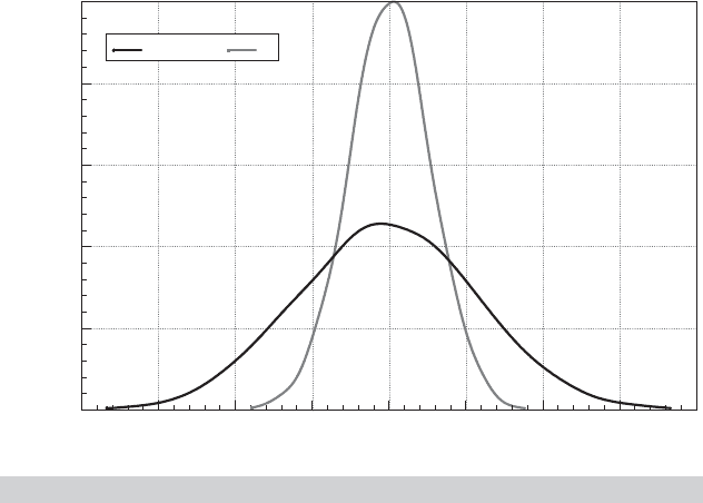
FIGURE 15.1

Distributions of Test Statistics.

We also computed a conﬁdence interval for the coefﬁcient on Ed using the conventional,

symmetric approach, b

± 1.96s(b

), and the percentile method in (15-7)–(15-8). The two

intervals are

Conventional: 0.051583 to 0.061825

Percentile: 0.045560 to 0.067909

Not surprisingly (given the larger standard errors), the percentile method gives a much wider

interval. Figure 15.1 shows a kernel density estimator of the distribution of the t statistics

computed using (15-7). It is substantially wider than the (approximate) standard normal den-

sity shown with it. This demonstrates the impact of the latent effect of the clustering on the

standard errors, and ultimately on the test statistic used to compute the conﬁdence intervals.

15.5 MONTE CARLO STUDIES

Simulated data generated by the methods of the preceding sections have various uses

in econometrics. One of the more common applications is the analysis of the properties

of estimators or in obtaining comparisons of the properties of estimators. For exam-

ple, in time-series settings, most of the known results for characterizing the sampling

distributions of estimators are asymptotic, large-sample results. But the typical time

series is not very long, and descriptions that rely on T, the number of observations,

going to inﬁnity may not be very accurate. Exact ﬁnite-sample properties are usually

intractable, however, which leaves the analyst with only the choice of learning about

the behavior of the estimators experimentally.

In the typical application, one would either compare the properties of two or more

estimators while holding the sampling conditions ﬁxed or study how the properties of

an estimator are affected by changing conditions such as the sample size or the value

of an underlying parameter.

616

PART III

✦

Estimation Methodology

Example 15.7 Monte Carlo Study of the Mean Versus the Median

In Example D.8, we compared the asymptotic distributions of the sample mean and the

sample median in random sampling from the normal distribution. The basic result is that

both estimators are consistent, but the mean is asymptotically more efﬁcient by a factor of

Asy. Var[Median]

Asy. Var[Mean]

= 1.5708.

This result is useful, but it does not tell which is the better estimator in small samples, nor does

it suggest how the estimators would behave in some other distribution. It is known that the

mean is affected by outlying observations whereas the median is not. The effect is averaged

out in large samples, but the small-sample behavior might be very different. To investigate

the issue, we constructed the following experiment: We sampled 500 observations from the

t distribution with d degrees of freedom by sampling d + 1 values from the standard normal

distribution and then computing

ir,d+1



l =1

ir,l

, i = 1, ..., 500, r = 1, ..., 100.

The t distribution with a low value of d was chosen because it has very thick tails and because

large outlying values have high probability. For each value of d, we generated R = 100

replications. For each of the 100 replications, we obtained the mean and median. Because

both are unbiased, we compared the mean squared errors around the true expectations using

(1/R)



r =1

(median

− 0)

(1/R)



r =1

(¯x

− 0)

We obtained ratios of 0.6761, 1.2779, and 1.3765 for d = 3, 6, and 10, respectively. (You

might want to repeat this experiment with different degrees of freedom.) These results agree

with what intuition would suggest. As the degrees of freedom parameter increases, which

brings the distribution closer to the normal distribution, the sample mean becomes more

efﬁcient—the ratio should approach its limiting value of 1.5708 as d increases. What might

be surprising is the apparent overwhelming advantage of the median when the distribution

is very nonnormal even in a sample as large as 500.

The preceding is a very small application of the technique. In a typical study, there

are many more parameters to be varied and more dimensions upon which the results

are to be studied. One of the practical problems in this setting is how to organize the

results. There is a tendency in Monte Carlo work to proliferate tables indiscriminately.

It is incumbent on the analyst to collect the results in a fashion that is useful to the

reader. For example, this requires some judgment on how ﬁnely one should vary the

parameters of interest. One useful possibility that will often mimic the thought process

of the reader is to collect the results of bivariate tables in carefully designed contour

plots.

There are any number of situations in which Monte Carlo simulation offers the

only method of learning about ﬁnite-sample properties of estimators. Still, there are a

number of problems with Monte Carlo studies. To achieve any level of generality, the

number of parameters that must be varied and hence the amount of information that

must be distilled can become enormous. Second, they are limited by the design of the

experiments, so the results they produce are rarely generalizable. For our example, we

may have learned something about the t distribution, but the results that would apply

in other distributions remain to be described. And, unfortunately, real data will rarely

conform to any speciﬁc distribution, so no matter how many other distributions we

CHAPTER 15

✦

Simulation-Based Estimation and Inference

617

analyze, our results would still only be suggestive. In more general terms, this problem

of speciﬁcity [Hendry (1984)] limits most Monte Carlo studies to quite narrow ranges

of applicability. There are very few that have proved general enough to have provided

a widely cited result.

15.5.1 A MONTE CARLO STUDY: BEHAVIOR OF A TEST STATISTIC

Monte Carlo methods are often used to study the behavior of test statistics when their

true properties are uncertain. This is often the case with Lagrange multiplier statistics.

For example, Baltagi (2005) reports on the development of several new test statistics for

panel data models such as a test for serial correlation. Examining the behavior of a test

statistic is fairly straightforward. We are interested in two characteristics: the true size of

the test—that is, the probability that it rejects the null hypothesis when that hypothesis

is actually true (the probability of a type 1 error) and the power of the test—that is the

probability that it will correctly reject a false null hypothesis (one minus the probability

of a type 2 error). As we will see, the power of a test is a function of the alternative

against which the null is tested.

To illustrate a Monte Carlo study of a test statistic, we consider how a familiar

procedure behaves when the model assumptions are incorrect. Consider the linear

regression model

= α + β x

+ γ z

+ ε

,ε

|(x

, z

) ∼ N[0,σ

The Lagrange multiplier statistic for testing the null hypothesis that γ equals zero for

this model is

LM = e



X(X



−1



/(e



/n)

where X = (1, x, z) and e

is the vector of least squares residuals obtained from the

regression of y on the constant and x (and not z). (See Section 14.6.3.) Under the

assumptions of the preceding model, above, the large sample distribution of the LM

statistic is chi-squared with one degree of freedom. Thus, our testing procedure is to

compute LM and then reject the null hypothesis γ = 0 if LM is greater than the critical

value. We will use a nominal size of 0.05, so the critical value is 3.84. The theory for

the statistic is well developed when the speciﬁcation of the model is correct. [See, for

example, Godfrey (1988).] We are interested in two speciﬁcation errors. First, how

does the statistic behave if the normality assumption is not met? Because the LM

statistic is based on the likelihood function, if some distribution other than the normal

governs ε

, then the LM statistic would not be based on the OLS estimator. We will

examine the behavior of the statistic under the true speciﬁcation that ε

comes from

a t distribution with ﬁve degrees of freedom. Second, how does the statistic behave

if the homoscedasticity assumption is not met? The statistic is entirely wrong if the

disturbances are heteroscedastic. We will examine the case in which the conditional

variance is Var[ε

|(x

, z

)] = σ

[exp(0.2x

)]

The design of the experiment is as follows: We will base the analysis on a sample

of 50 observations. We draw 50 observations on x

and z

from independent N[0, 1]

populations at the outset of each cycle. For each of 1,000 replications, we draw a sample

of 50 ε

’s according to the assumed speciﬁcation. The LM statistic is computed and the

Two that have withstood the test of time are Griliches and Rao (1969) and Kmenta and Gilbert (1968).

618

PART III

✦

Estimation Methodology

TABLE 15.4

Size and Power Functions for LM Test

Gamma

0.0 0.1 0.2 0.3 0.4 0.5 0.6 0.7 0.8 0.9 1.0

Model −0.1 −0.2 −0.3 −0.4 −0.5 −0.6 −0.7 −0.8 −0.9 −1.0

Normal 0.059 0.090 0.235 0.464 0.691 0.859 0.957 0.989 0.998 1.000 1.000

0.103 0.236 0.451 0.686 0.863 0.961 0.989 0.999 1.000 1.000

t (5) 0.052 0.083 0.169 0.320 0.508 0.680 0.816 0.911 0.956 0.976 0.994

0.080 0.177 0.312 0.500 0.677 0.822 0.921 0.953 0.984 0.993

Het. 0.071 0.098 0.249 0.457 0.666 0.835 0.944 0.984 0.995 0.998 1.000

0.107 0.239 0.442 0.651 0.832 0.940 0.985 0.996 1.000 1.000

proportion of the computed statistics that exceed 3.84 is recorded. The experiment is

repeated for γ = 0 to ascertain the true size of the test and for values of γ including

−1,...,−0.2, −0.1, 0, 0.1, 0.2,...,1.0 to assess the power of the test. The cycle of tests

is repeated for the two scenarios, the t (5) distribution and the model with hetero-

scedasticity.

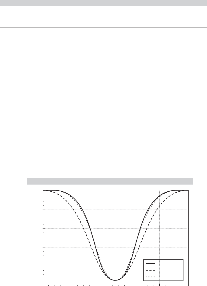
Table 15.4 lists the results of the experiment. The ﬁrst row shows the expected

results for the LM statistic under the model assumptions for which it is appropriate.

The size of the test appears to be in line with the theoretical results. Comparing the ﬁrst

and third rows, it appears that the presence of heteroscedasticity seems not to degrade

the power of the statistic. But the different distributional assumption does. Figure 15.2

plots the values in the table, and displays the characteristic form of the power function

for a test statistic.

FIGURE 15.2

Power Functions.

0.00

1.00 0.60

Power

Gamma

0.20 0.20 0.60 1.00

0.20

0.40

0.60

0.80

1.00

POWER_N

POWER_T5

POWER_H