Greene W.H. Econometric Analysis

Подождите немного. Документ загружается.

CHAPTER 15

✦

Simulation-Based Estimation and Inference

639

estimate of  is shown here.

 =

0.04114 000000

0.00715 0.07266 00000

−0.02446 0.12392 0.07247 0 0 0 0

0.09972 −0.00644 0.31916 0.07614 0 0 0

−0.08928 0.02143 −0.25105 0.07583 0.04053 0 0

0.03842 −0.06321 −0.03992 −0.06693 −0.05490 0.00857 0

−0.00833 −0.00257 −0.02478 0.01594 0.00102 −0.00185 0.0018.

An estimate of the correlation matrix for the parameters might also be informative. This is also

derived from

 by computing

 =





and then transforming the covariances to correlations

by dividing by the products of the respective standard deviations (the values in parentheses

in Table 15.7). The result is

R =

0.0979 1

−0.1680 0.83040 1

0.2907 0.00980 0.3983 1

−0.3180 0.04481 −0.3266 −0.8659 1

0.3176 −0.48890 −0.6622 −0.3277 −0.06073 1

−0.2700 −0.10940 −0.4253 −0.7097 0.94190 −0.08228 1.

15.8 HIERARCHICAL LINEAR MODELS

Example 11.20 examined an application of a “two-level model,” or “hierarchical model,”

for mortgage rates,

= β

+ β

2,i

+ various terms relating to the mortgate + ε

The second level equation is

2,i

= α

+ α

GFA

+ α

one-year treasury rate + α

ten-year treasure rate

+α

credit risk + α

prepayment risk +···+u

Recent research in many ﬁelds has extended the idea of hierarchical modeling to the

full set of parameters in the model. (Depending on the ﬁeld studied, the reader may

ﬁnd these labeled “hierarchical models,” mixed models, “random parameters models,”

or “random effects models.” The last of these generalizes our notion of random effects.)

A two-level formulation of the model in (15-34) might appear as

= x



+ ε

= β + z

+ u

(A three-level model is shown in Example 15.14.) This model retains the earlier stochas-

tic speciﬁcation but adds the measurement equation to the generation of the random

parameters. In principle, this is actually only a minor extension of the model used thus

far. The model of the previous section now becomes

= x



(β + z

+ w

) + ε

which is essentially the same as our earlier model in (15-28)–(15-31) with the addition

of product (interaction) terms of the form δ

itk

, which suggests how it might be

640

PART III

✦

Estimation Methodology

estimated (simply by adding the interaction terms to the previous formulation). In the

template in (15-26), the term σ

becomes x



(z

+ w

), θ = (β



, δ



, λ



,σ

)



where



is a row vector composed of the rows of , and λ



is a row vector composed of the

rows of . The scalar term w

in the derivatives is replaced by a column vector of terms

contained in (x

⊗ z

, x

⊗ w

The hierarchical model can be extended in several useful directions. Recent analyses

have expanded the model to accommodate multilevel stratiﬁcation in data sets such as

those we considered in the treatment of nested random effects in Section 14.9.6.b. A

three-level model would appear as in the next example that relates to home sales,

ijt

= x



ijt

+ ε

, t = site, j = neighborhood, i = community,

= β

+ z

+ u

(15-35)

= π + r

+ v

Example 15.14 Hierarchical Linear Model of Home Prices

Beron, Murdoch, and Thayer (1999) used a hedonic pricing model to analyze the sale

prices of 76,343 homes in four California counties: Los Angeles, San Bernardino, Riverside,

and Orange. The data set is stratiﬁed into 2,185 census tracts and 131 school districts. Home

prices are modeled using a three-level random parameters pricing model. (We will change

their notation somewhat to make roles of the components of the model more obvious.) Let

site denote the speciﬁc location (sale), nei denote the neighborhood, and com denote the

community, the highest level of aggregation. The pricing equation is

ln Price

site,nei,com

= π

nei,com



k=1

nei,com

k,site,nei,com

+ ε

site,nei,com

nei,com

= β

0,k

com



l =1

l ,k

com

k,nei,com

nei,com

, k = 0, ..., K ,

l ,k

com

= γ

0,l.k



m=1

m,l,k

m,com

+ u

l ,k

com

, l = 1, ..., L.

There are K level-one variables, x

, and a constant in the main equation, L level-two variables,

, and a constant in the second-level equations, and M level-three variables, e

, and a

constant in the third-level equations. The variables in the model are as follows. The level-one

variables deﬁne the hedonic pricing model,

x = house size, number of bathrooms, lot size, presence of central heating,

presence of air conditioning, presence of a pool, quality of the view,

age of the house, distance to the nearest beach.

Levels two and three are measured at the neighborhood and community levels

z = percentage of the neighborhood below the poverty line,

racial makeup of the neighborhood,

percentage of residents over 65,

average time to travel to work

and

e = FBI crime index, average achievement test score in school district,

air quality measure, visibility index.

The model is estimated by maximum simulated likelihood.

CHAPTER 15

✦

Simulation-Based Estimation and Inference

641

The hierarchical linear model analyzed in this section is also called a “mixed model”

and “random parameters” model. Although the three terms are usually used inter-

changeably, each highlights a different aspect of the structural model in (15-35). The

“hierarchical” aspect of the model refers to the layering of coefﬁcients that is built into

stratiﬁed and panel data structures, such as in Example 15.4. The random parameters

feature is a signature feature of the model that relates to the modeling of heterogeneity

across units in the sample. Note that the model in (15-35) and Beron et al.’s applica-

tion could be formulated without the random terms in the lower-level equations. This

would then provide a convenient way to introduce interactions of variables in the linear

regression model. The addition of the random component is motivated on precisely the

same basis that u

appears in the familiar random effects model in Section 11.5 and

(15-39). It is important to bear in mind, in all these structures, strict mean independence

is maintained between u

, and all other variables in the model. In most treatments, we

go yet a step further and assume a particular distribution for u

, typically joint nor-

mal. Finally, the “mixed” model aspect of the speciﬁcation relates to the underlying

integration that removes the heterogeneity, for example, in (15-13). The unconditional

estimated model is a mixture of the underlying models, where the weights in the mixture

are provided by the underlying density of the random component.

15.9 NONLINEAR RANDOM PARAMETER MODELS

Most of the preceding applications have used the linear regression model to illustrate

and demonstrate the procedures. However, the template used to build the model has

no intrinsic features that limit it to the linear regression. The initial description of the

model and the ﬁrst example were applied to a nonlinear model, the Poisson regression.

We will examine a random parameters binary choice model in the next section as well.

This random parameters model has been used in a wide variety of settings. One of the

most common is the multinomial choice models that we will discuss in Chapter 18.

The simulation-based random parameters estimator/model is extremely ﬂexible.

[See Train and McFadden (2000) for discussion.] The simulation method, in addition

to extending the reach of a wide variety of model classes, also allows great ﬂexibility in

terms of the model itself. For example, constraining a parameter to have only one sign

is a perennial issue. Use of a lognormal speciﬁcation of the parameter, β

= exp(β +

σ w

) provides one method of restricting a random parameter to be consistent with a

theoretical restriction. Researchers often ﬁnd that the lognormal distribution produces

unrealistically large values of the parameter. A model with parameters that vary in a

restricted range that has found use is the random variable with symmetric about zero

triangular distribution,

f (w) = 1[−a ≤ w ≤ 0](a + w)/a

+ 1[0 < w ≤ a](a − w)/a

A draw from this distribution with a = 1 can be computed as

w = 1[u ≤ .5][(2u)

1/2

− 1] + 1[u >.5][1 − (2(1 − u))

1/2

where u is the U[0, 1] draw. Then, the parameter restricted to the range β ±λ is obtained

as β +λw. A further reﬁnement to restrict the sign of the random coefﬁcient is to force

λ = β, so that β

ranges from 0 to 2λ. [Discussion of this sort of model construction is

642

PART III

✦

Estimation Methodology

given in Train and Sonnier (2003) and Train (2009).] There is a large variety of methods

for simulation that allow the model to be extended beyond the linear model and beyond

the simple normal distribution for the random parameters.

Random parameters models have been implemented in several contemporary com-

puter packages. The PROC MIXED package of routines in SAS uses a kind of general-

ized least squares for linear, Poisson, and binary choice models. The GLAMM program

[Rabe-Hesketh, Skrondal, and Pickles (2005)] written for Stata uses quadrature meth-

ods for several models including linear, Poisson, and binary choice. The RPM and RPL

procedures in LIMDEP/NLOGIT use the methods described here for linear, binary

choice, censored data, multinomial, ordered choice, and several others. Finally, the ML-

Win package (http://cmm.bristol.ac.uk/MLwiN/) is a large implementation of some of

the models discussed here. MLWin uses MCMC methods with noninformative priors to

carry out maximum simulated likelihood estimation.

15.10 INDIVIDUAL PARAMETER ESTIMATES

In our analysis of the various random parameters speciﬁcations, we have focused on

estimation of the population parameters, β, , and  in the model,

= β + z

+ w

for example, in Example 15.13, where we estimated β and  in a model of production.

At a few points, it is noted that it might be useful to estimate the individual speciﬁc β

We did a similar exercise in analyzing the Hildreth/Houck/Swamy model in Example

11.19 in Section 11.11.1. The model is

= X

+ ε

= β + u

where no restriction is placed on the correlation between u

and X

. In this “ﬁxed effects”

case, we obtained a feasible GLS estimator for the population mean, β,

β =



i=1

where



i=1



 + ˆσ



)

−1



−1



 + ˆσ



)

−1



−1

and

= (X



)

−1



For each group, we then proposed an estimator of E[β

| information in hand about

group i]as

Est. E[β

, X

] = b

(

β − b

)

where





)



−1



−1



−1

. (15-36)

CHAPTER 15

✦

Simulation-Based Estimation and Inference

643

The estimator of E[β

, X

] is equal to the least squares estimator plus a proportion

of the difference between

β and b

. (The matrix

is between 0 and I. If there were a

single column in X

, then ˆq

would equal (1/ ˆγ)/{(1/ ˆγ)+ [1/(s



)]}.)

We can obtain an analogous result for the mixed models we have examined in this

chapter. [See Train (2003).] From the initial model assumption, we have

f (y

, β

, θ )

where

= β + z

+ w

(15-37)

and θ is any other parameters in the model, such as σ

in the linear regression model.

For a panel, since we are conditioning on β

, that is, on w

, the T

observations are

independent, and it follows that

f (y

, y

,...,y

iTi

, β

, θ ) = f (y

, β

, θ ) = 

f (y

, β

, θ ). (15-38)

This is the contribution of group i to the likelihood function (not its log) for the sample,

given β

; that is, note that the log of this term is what appears in the simulated log

likelihood function in (15-31) for the normal linear model and in (15-16) for the Poisson

model. The marginal density for β

is induced by the density of w

in (15-37). For

example, if w

is joint normally distributed, then f (β

) = N[β +z

, 



]. As we noted

earlier in Section 15.9, some other distribution might apply. Write this generically as

the marginal density of β

, f (β

, ), where  is the parameters of the underlying

distribution of β

, for example (β, , ) in (15-37). Then, the joint distribution of y

and β

f (y

, β

, z

, θ , ) = f (y

, β

, θ ) f (β

, ).

We will now use Bayes’s theorem to obtain f (β

, X

, z

, θ , ):

f (β

, X

, z

, θ , ) =

f (y

, β

, θ ) f (β

, )

f (y

, z

, θ , )

f (y

, β

, θ ) f (β

, )

f (y

, β

, z

, θ ,)dβ

f (y

, β

, θ ) f (β

, )

f (y

, β

, θ ) f (β

, )dβ

The denominator of this ratio is the integral of the term that appears in the log-likelihood

conditional on β

. We will return momentarily to computation of the integral. We now

have the conditional distribution of β

, X

, z

, θ , . The conditional expectation of

, X

, z

, θ ,  is

E[β

, X

, z

, θ , ] =

f (y

, β

, θ ) f (β

, )

f (y

, β

, θ ) f (β

, )dβ

644

PART III

✦

Estimation Methodology

Neither of these integrals will exist in closed form. However, using the methods already

developed in this chapter, we can compute them by simulation. The simulation estimator

will be

Est .E[β

, X

, z

, θ , ] =

(1/R)



r=1

t=1

f (y

θ)

(1/R)



r=1

t=1

f (y

θ)



r=1

(15-39)

where

is deﬁned in (15-20)–(15-21) and

β +

z

+ w

This can be computed after the estimation of the population parameters. (It may be

more efﬁcient to do this computation during the iterations, since everything needed to

do the calculation will be in place and available while the iterations are proceeding.)

For example, for the random parameters linear model, we will use

f (y

θ) =

ˆσ

√

2π

exp



−



− x



(

β +

z

w

)



2ˆσ



. (15-40)

We can also estimate the conditional variance of β

by estimating ﬁrst, one element at

a time, E[β

i,k

, X

, z

, θ , ], then, again one element at a time

Est.Var [β

i,k

, X

, z

, θ , ] =



Est. E[β

i,k

, X

, z

, θ , ]



−



Est. E[β

i,k

, X

, z

, θ , ]



(15-41)

With the estimates of the conditional mean and conditional variance in hand, we can

then compute the limits of an interval that resembles a conﬁdence interval as the mean

plus and minus two estimated standard deviations. This will construct an interval that

contains at least 95 percent of the conditional distribution of β

Some aspects worth noting about this computation are as follows:

•

The preceding suggested interval is a classical (sampling-theory-based) counter-

part to the highest posterior density interval that would be computed for β

for a

hierarchical Bayesian estimator.

•

The conditional distribution from which β

is drawn might not be symmetric or

normal, so a symmetric interval of the mean plus and minus two standard deviations

may pick up more or less than 95 percent of the actual distribution. This is likely

to be a small effect. In any event, in any population, whether symmetric or not,

the mean plus and minus two standard deviations will typically encompass at least

95 percent of the mass of the distribution.

•

It has been suggested that this classical interval is too narrow because it does not

account for the sampling variability of the parameter estimators used to construct

it. But, the suggested computation should be viewed as a “point” estimate of the

interval, not an interval estimate as such. Accounting for the sampling variability

of the estimators might well suggest that the endpoints of the interval should be

somewhat farther apart. The Bayesian interval that produces the same estimation

CHAPTER 15

✦

Simulation-Based Estimation and Inference

645

would be narrower because the estimator is posterior to, that is, applies only to the

sample data.

•

Perhaps surprisingly so, even if the analysis departs from normal marginal distri-

butions β

, the sample distribution of the n estimated conditional means is not

necessarily normal. Kernel estimators based on the n estimators, for example, can

have a variety of shapes.

•

A common misperception found in the Bayesian and classical literatures alike is that

the preceding produces an estimator of β

. In fact, it is an estimator of conditional

mean of the distribution from which β

is an observation. By construction, for

example, every individual with the same (y

. X

, z

) has the same prediction even

though the w

and any other stochastic elements of the model, such as ε

, will differ

across individuals.

Example 15.15 Individual State Estimates of Private Capital Coefﬁcient

Example 15.13 presents feasible GLS and maximum simulated likelihood estimates of

Munnell’s state production model. We have computed the estimates of E[β

, X

] for the

48 states in the sample using (15-36) for the ﬁxed effects estimates and (15-39) for the ran-

dom effects estimates. Figures 15.6 and 15.7 examine the estimated coefﬁcients for private

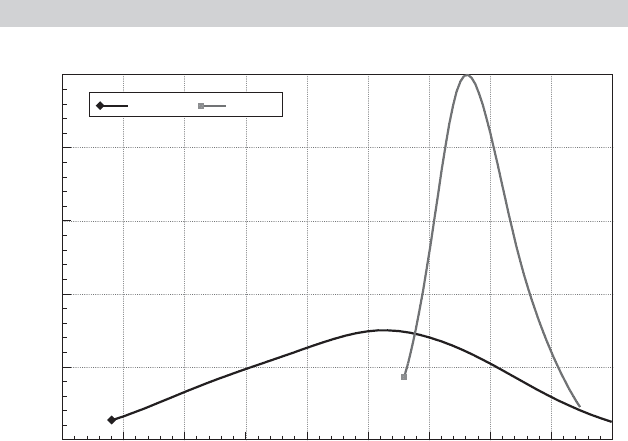
capital. Figure 15.6 displays kernel density estimates for the population distributions based

on the ﬁxed and random effects estimates computed using (15-36) and (15-39). The much

narrower distribution corresponds to the random effects estimates. The substantial overall

difference of the distributions is presumably due in large part to the difference between the

ﬁxed effects and random effects assumptions. One might suspect on this basis that the ran-

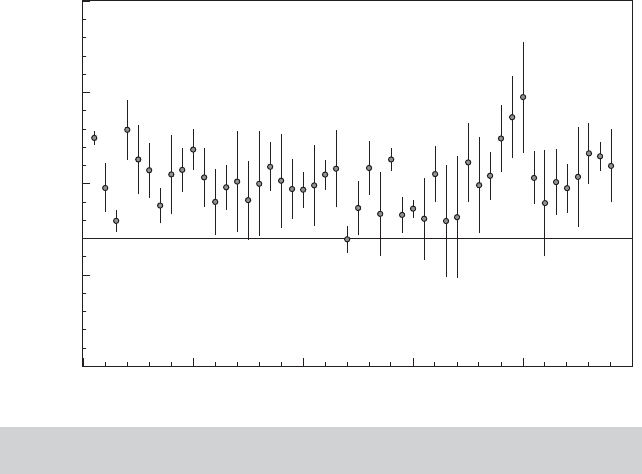
dom effects assumption is restrictive. Figure 15.7 shows the results based on the random

parameters model, using (15-39) and (15-41) to compute the estimates. As expected, the

range of variation of the estimators in the conditional distributions is much smaller than the

overall range of variation shown in Figure 15.6.

FIGURE 15.6

Kernel Density Estimates of Parameter Distributions.

Range(x)

Kernel Density Estimates

1.21

2.42

3.64

4.85

6.06

0.00

0.30 0.20 0.10 0.00 0.10 0.20 0.30 0.40 0.50

0.40

Density

B2FE B2RP

646

PART III

✦

Estimation Methodology

State Number

95% Intervals of Conditional Distributions of b(PC)

0.3100

0.3150

0.3200

0.3250

0.3050

10 20 30 40 500

Limits of Conditional Distributions

FIGURE 15.7

Estimates of Conditional Distributions for Private

Capital Coefﬁcient.

Example 15.16 Mixed Linear Model for Wages

Koop and Tobias (2004) analyzed a panel of 17,919 observations in their study of the rela-

tionship between wages and education, ability and family characteristics. (See the end of

chapter applications in Chapters 3 and 5 and Appendix Table F3.2 for details on the location

of the data.) The variables used in the analysis are

Person id

Education (time varying)

Log of hourly wage (time varying)

Potential experience (time varying)

Time trend (time varying)

Ability (time invariant)

Mother’s education (time invariant)

Father’s education (time invariant)

Dummy variable for residence in a broken home (time invariant)

Number of siblings (time invariant)

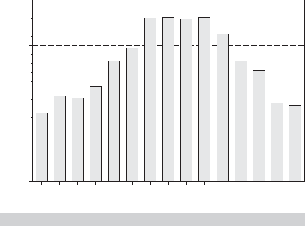
This is an unbalanced panel of 2,178 individuals; Figure 15.8 shows a frequency count of

the numbers of observations in the sample. We will estimate the following hierarchical wage

model

ln Wage

= β

1,i

+ β

2,i

Education

+ β

Experience

+ β

Experience

+ β

Broken Home

+ β

Siblings

+ ε

1,i

= α

1,1

+ α

1,2

Ability

+ α

1,3

Mother’s education

+ α

1,4

Father’s education

+ u

1,i

2,i

= α

2,1

+ α

2,2

Ability

+ α

2,3

Mother’s education

+ α

2,4

Father’s education

+ u

2,i

CHAPTER 15

✦

Simulation-Based Estimation and Inference

647

1234

224

168

112

Frequency

6 7 8 9 10 11 12 135

NUM_OBS

14 15

FIGURE 15.8

Group Sizes for Wage Data Panel.

Estimates are computed using the maximum simulated likelihood method described in

Sections 15.6.3 and 15.7. Estimates of the model parameters appear in Table 15.8. The

four models in Table 15.8 are the pooled OLS estimates, the random effects model, and

the random parameters models, ﬁrst assuming that the random parameters are uncorrelated

(

= 0) and then allowing free correlation (

= nonzero). The differences between the

conventional and the robust standard errors in the pooled model are fairly large, which sug-

gests the presence of latent common effects. The formal estimates of the random effects

model conﬁrm this. There are only minor differences between the FGLS and the ML estimates

of the random effects model. But, the hypothesis of the pooled model is soundly rejected by

the likelihood ratio test. The LM statistic [Section 11.5.4 and (11-42)] is 11,709.7, which is far

larger than the critical value of 3.84. So, the hypothesis of the pooled model is ﬁrmly rejected.

The likelihood ratio statistic based on the MLEs is 2( 10, 840.18 −(−885.674) ) = 23, 451.71,

which produces the same conclusion. An alternative approach would be to test the hypoth-

esis that σ

= 0 using a Wald statistic—the standard t test. The software used for this exer-

cise reparameterizes the log-likelihood in terms of θ

= σ

/σ

and θ

= 1/σ

. One approach,

based on the delta method (see Section 4.4.4), would be to estimate σ

with the MLE of θ

/θ

The asymptotic variance of this estimator would be estimated using Theorem 4.5. Alterna-

tively, we might note that σ

must be positive in this model, so it is sufﬁcient simply to test the

hypothesis that θ

= 0. Our MLE of θ

is 0.999206 and the estimated asymptotic standard

error is 0.03934. Following this logic, then, the test statistic is 0.999206/0.03934 = 25.397.

This is far larger than the critical value of 1.96, so, once again, the hypothesis is rejected.

We do note a problem with the LR and Wald tests. The hypothesis that σ

= 0 produces

a nonstandard test under the null hypothesis, because σ

= 0 is on the boundary of the

parameter space. Our standard theory for likelihood ratio testing (see Chapter 14) requires

the restricted parameters to be in the interior of the parameter space, not on the edge. The

distribution of the test statistic under the null hypothesis is not the familiar chi squared. This

issue is confronted in Breusch and Pagan (1980) and Godfrey (1988) and analyzed at (great)

length by Andrews (1998, 1999, 2000, 2001, 2002) and Andrews and Ploberger (1994, 1995).

The simple expedient in this complex situation is to use the LM statistic, which remains

consistent with the earlier conclusion.

648

PART III

✦

Estimation Methodology

TABLE 15.8

Estimated Random Parameter Models

Random Effects FGLS Random Random

Pooled OLS

[Random Effects MLE] Parameters Parameters

Std.Err. Estimate Std.Err. Estimate Estimate

Variable Estimate

(Robust)[MLE][MLE](Std.Err.)(Std.Err.)

Exp 0.04157 0.001819 0.04698 0.001468 0.04758 0.04802

(0.002242) [0.04715] [0.001481] (0.001108) (0.001118)

Exp

−0.00144 0.0001002 −0.00172 0.0000805 −0.001750 −0.001761

(0.000126) [−0.00172] [0.000081] (0.000063) (0.0000631)

Broken −0.02781 0.005296 −0.03185 0.01089 −0.01236 −0.01980

(0.01074) [−0.03224] [0.01172] (0.003669) (0.003534)

Sibs −0.00120 0.0009143 −0.002999 0.001925 0.0000496 −0.001953

(0.001975) [−0.00310] [0.002071] (0.000662) (0.0006599)

Constant 0.09728 0.01589 0.03281 0.02438 0.3277 0.3935

(0.02783) [0.03306] [0.02566] (0.03803) (0.03778)

Ability 0.04232 0.1107

(0.01064) (0.01077)

MEd −0.01393 −0.02887

(0.0040) (0.003990)

FEd −0.007548 0.002657

(0.003252) (0.003299)

0.172278 0.004187 0.5026

[0.18767] (0.001320)

Educ 0.03854 0.001040 0.04072 0.001758 0.01253 0.007607

(0.002013) [0.04061] [0.001853] (0.003015) (0.002973)

Ability −0.0002560 −0.005316

(0.000869) (0.0008751)

MEd 0.001054 0.002142

(0.000321) (0.0003165)

Fed 0.0007754 0.00006752

(0.000255) (0.00001354)

0.01622 0.03365

(0.000114)

u,12

0.0000 −0.01560

0.0000 −0.92259

0.2542736 0.187017 0.192741 0.1919182

[0.187742]



0.004187 0.5026

(0.001320) (0.008775)

0.0000 −0.03104



(0) (0.0001114)

0.01622 0.01298



(0.000113) (0.0006841)

ln L −885.6740 [10480.18] 3550.594 3587.611