Greene W.H. Econometric Analysis

Подождите немного. Документ загружается.

CHAPTER 15

✦

Simulation-Based Estimation and Inference

649

The third and fourth models in Table 15.8 present the mixed model estimates. The ﬁrst of

them imposes the restriction that 

= 0, or that the two random parameters are uncorre-

lated. The second mixed model allows 

to be a free parameter. The implied estimators

for σ

, σ

and σ

u,21

are the elements of 



,or

= 

u,21

= 



= 

+ 

These estimates are shown separately in the table. Note that in all three random parame-

ters models (including the random effects model which is equivalent to the mixed model

with all α

= 0 save for α

1,1

and α

2,1

as well as 

= 

= 0.0), the estimate of

is relatively unchanged. The three models decompose the variation across groups in

the parameters differently, but the overall variation of the dependent variable is largely the

same.

The interesting coefﬁcient in the model is β

2,i

. Reading across the row for Educ, one

might suspect that the random parameters model has washed out the impact of education,

since the “coefﬁcient” declines from 0.04072 to 0.007607. However, in the mixed models,

the “mean” parameter, α

2,1

, is not the coefﬁcient of interest. The coefﬁcient on education in

the model is β

2,i

= α

2,1

+α

2,2

Ability +β

2,3

Mother’s education +β

2,4

Father’s education +u

2,i

A rough indication of the magnitude of this result can be seen by inserting the sample means

for these variables, 0.052374, 11.4719, and 11.7092, respectively. With these values, the

mean value for the education coefﬁcient is approximately 0.0327. This is comparable, though

somewhat smaller, than the estimates for the pooled and random effects model. Of course,

variation in this parameter across the sample individuals was the objective of this speciﬁca-

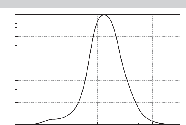
tion. Figure 15.9 plots a kernel density estimate for the estimated conditional means for the

2,178 sample individuals. The ﬁgure shows the very wide range of variation in the sample

estimates.

FIGURE 15.9

Kernel Density Estimate for Education Coefﬁcient.

0.000 0.010 0.020 0.0400.030

␤

Educ, i

Density

0.050 0.060

650

PART III

✦

Estimation Methodology

15.11 MIXED MODELS AND LATENT CLASS

MODELS

Sections 15.7–15-10 examined different approaches to modeling parameter heterogene-

ity. The ﬁxed effects approach begun in Section 11.4 is extended to include the full set

of regression coefﬁcients in Section 11.11.1. where

= X

+ ε

= β + u

and no restriction is placed on E[u

]. Estimation produces a feasible GLS estimate

of β. Estimation of β begins with separate least squares estimation with each group,

i—because of the correlation between u

and x

, the pooled estimator is not consis-

tent. The efﬁcient estimator of β is then a mixture of the bi’s. We also examined an

estimator of β

, using the optimal predictor from the conditional distributions, (15-39).

The crucial assumption underlying the analysis is the possible correlation between X

and u

. We also considered two modiﬁcations of this random coefﬁcients model. First,

a restriction of the model in which some coefﬁcients are nonrandom provides a useful

simpliﬁcation. The familiar ﬁxed effects model of Section 11.4 is such a case, in which

only the constant term varies across individuals. Second, we considered a hierarchical

form of the model

= β + z

+ u

. (15-42)

This approach is applied to an analysis of mortgage rates in Example 11.20. [Pl ¨umper

and Troeger’s (2007) FEVD estimator examined in Section 11.4.5 is essentially this

model as well.]

A second approach to random parameters modeling builds from the crucial assump-

tion added to (15-42) that u

and X

are uncorrelated. The general model is deﬁned in

terms of the conditional density of the random variable, f (y

, β

, θ ), and the marginal

density of the random coefﬁcients, f (β

, ), in which  is the separate parameters of

this distribution. This leads to the mixed models examined in this chapter. The random

effects model that we examined in Section 11.5 and several other points is a special

case in which only the constant term is random (like the ﬁxed effects model). We also

considered the speciﬁc case in which u

is distributed normally with variance σ

A third approach to modeling heterogeneity in parametric models is to use a

discrete distribution, either as an approximation to an underlying continuous distri-

bution, or as the model of the data generating process in its own right. (See Sec-

tion 14.10.) This model adds to the preceding a nonparametric speciﬁcation of the

variation in β

Prob(β

= β

) = π

, j = 1,..., J.

A somewhat richer, semiparametric form that mimics (15-42) is

Prob(β

= β

) = π

, ), j = 1,...,J.

We continue to assume that the process generating variation in β

across individuals is

independent of the process that produces X

—that is, in a broad sense, we retain the

random effects approach. This latent class model is gaining popularity in the current

CHAPTER 15

✦

Simulation-Based Estimation and Inference

651

TABLE 15.9

Estimated Random Parameters Model

Probit RP Mean RP Std. Dev. Empirical Distn.

Constant −1.96 −3.91 2.70 −3.27

(0.23) (0.20) (0.57)

In Sales 0.18 0.36 0.28 0.32

(0.022) (0.019) (0.15)

Relative Size 1.07 6.01 5.99 3.33

(0.14) (0.22) (2.25)

Import 1.13 1.51 0.84 2.01

(0.15) (0.13) (0.58)

FDI 2.85 3.81 6.51 3.76

(0.40) (0.33) (1.69)

Productivity −2.34 −5.10 13.03 −8.15

(0.72) (0.73) (8.29)

Raw materials −0.28 −0.31 1.65 −0.18

(0.081) (0.075) (0.57)

Investment 0.19 0.27 1.42 0.27

(0.039) (0.032) (0.38)

ln L −4114.05 −3498.654

literature. In the last example of this chapter, we will examine a comparison of mixed

and ﬁnite mixture models for a nonlinear model.

Example 15.17 Maximum Simulated Likelihood Estimation of a Binary

Choice Model

Bertschek and Lechner (1998) analyzed the product innovations of a sample of German

manufacturing ﬁrms. They used a probit model (Sections 17.2–17.4) to study ﬁrm innovations.

The model is for Prob[y

= 1|x

, β

] where

= 1ifﬁrmi realized a product innovation in year t and 0 if not.

The independent variables in the model are

it,1

= constant,

it,2

= log of sales,

it,3

= relative size = ratio of employment in business unit to employment in the industry,

it,4

= ratio of industry imports to (industry sales + imports),

it,5

= ratio of industry foreign direct investment to (industry sales + imports),

it,6

= productivity = ratio of industry value added to industry employment,

it,7

= dummy variable indicating ﬁrm is in the raw materials sector,

it,8

= dummy variable indicating ﬁrm is in the investment goods sector.

The sample consists of 1,270 German ﬁrms observed for ﬁve years, 1984–1988. (See Ap-

pendix Table F15.1.) The density that enters the log-likelihood is

f ( y

, β

) = Prob[ y



] = [(2y

− 1)x



], y

= 0, 1,

where

= β + v

, v

∼ N[0, ].

To be consistent with Bertschek and Lechner (1998) we did not ﬁt any ﬁrm-speciﬁc time-

invariant components in the main equation for β

Table 15.9 presents the estimated

Apparently they did not use the second derivatives to compute the standard errors—we could not replicate

these. Those shown in the Table 15.9 are our results.

652

PART III

✦

Estimation Methodology

TABLE 15.10

Estimated Latent Class Model

Class 1 Class 2 Class 3 Posterior

Constant −2.32 −2.71 −8.97 −3.38

(0.59) (0.69) (2.20) (2.14)

In Sales 0.32 0.23 0.57 0.34

(0.061) (0.072) (0.18) (0.09)

Relative Size 4.38 0.72 1.42 2.58

(0.89) (0.37) (0.76) (1.30)

Import 0.94 2.26 3.12 1.81

(0.37) (0.53) (1.38) (0.74)

FDI 2.20 2.81 8.37 3.63

(1.16) (1.11) (1.93) (1.98)

Productivity −5.86 −7.70 −0.91 −5.48

(2.70) (4.69) (6.76) (1.78)

Raw Materials −0.11 −0.60 0.86 −0.08

(0.24) (0.42) (0.70) (0.37)

Investment 0.13 0.41 0.47 0.29

(0.11) (0.12) (0.26) (0.13)

ln L −3503.55

Class Prob (Prior) 0.469 0.331 0.200

(0.0352) (0.0333) (0.0246)

Class Prob (Posterior) 0.469 0.331 0.200

(0.394) (0.289) (0.325)

Pred. Count 649 366 255

coefﬁcients for the basic probit model in the ﬁrst column. These are the values reported

in the 1998 study. The estimates of the means, β, are shown in the second column. There

appear to be large differences in the parameter estimates, although this can be misleading as

there is large variation across the ﬁrms in the posterior estimates. The third column presents

the square roots of the implied diagonal elements of  computed as the diagonal elements of



. These estimated standard deviations are for the underlying distribution of the parameter

in the model—they are not estimates of the standard deviation of the sampling distribution of

the estimator. That is shown for the mean parameter in the second column. The fourth col-

umn presents the sample means and standard deviations of the 1,270 estimated conditional

estimates of the coefﬁcients.

The latent class formulation developed in Section 14.10 provides an alternative approach

for modeling latent parameter heterogeneity.

To illustrate the speciﬁcation, we will reesti-

mate the random parameters innovation model using a three-class latent class model. Esti-

mates of the model parameters are presented in Table 15.10. The estimated conditional mean

shown, which is comparable to the empirical means in the rightmost column in Table 15.9 for

the random parameters model, are the sample average and standard deviation of the 1,270

ﬁrm-speciﬁc posterior mean parameter vectors. They are computed using

= 

j =1

ˆπ

where ˆπ

is the conditional estimator of the class probabilities in (14-102). These estimates

differ considerably from the probit model, but they are quite similar to the empirical means in

Table 15.9. In each case, a conﬁdence interval around the posterior mean contains the one-

class pooled probit estimator. Finally, the (identical) prior and average of the sample posterior

class probabilities are shown at the bottom of the table. The much larger empirical standard

deviations reﬂect that the posterior estimates are based on aggregating the sample data and

involve, as well, complicated functions of all the model parameters. The estimated numbers

of class members are computed by assigning to each ﬁrm the predicted class associated

with the highest posterior class probability.

See Greene (2001) for a survey. For two examples, Nagin and Land (1993) employed the model to study

age transitions through stages of criminal careers and Wang et al. (1998) and Wedel et al. (1993) used the

Poisson regression model to study counts of patents.

CHAPTER 15

✦

Simulation-Based Estimation and Inference

653

15.12 SUMMARY AND CONCLUSIONS

This chapter has outlined several applications of simulation-assisted estimation and

inference. The essential ingredient in any of these applications is a random number

generator. We examined the most common method of generating what appear to be

samples of random draws from a population—in fact, they are deterministic Markov

chains that only appear to be random. Random number generators are used directly to

obtain draws from the standard uniform distribution. The inverse probability transfor-

mation is then used to transform these to draws from other distributions. We examined

several major applications involving random sampling:

•

Random sampling, in the form of bootstrapping, allows us to infer the characteris-

tics of the sampling distribution of an estimator, in particular its asymptotic variance.

We used this result to examine the sampling variance of the median in random sam-

pling from a nonnormal population. Bootstrapping is also a useful, robust method

of constructing conﬁdence intervals for parameters.

•

Monte Carlo studies are used to examine the behavior of statistics when the precise

sampling distribution of the statistic cannot be derived. We examined the behavior

of a certain test statistic and of the maximum likelihood estimator in a ﬁxed effects

model.

•

Many integrals that do not have closed forms can be transformed into expectations

of random variables that can be sampled with a random number generator. This

produces the technique of Monte Carlo integration. The technique of maximum

simulated likelihood estimation allows the researcher to formulate likelihood func-

tions (and other criteria such as moment equations) that involve expectations that

can be integrated out of the function using Monte Carlo techniques. We used the

method to ﬁt random parameters models.

The techniques suggested here open up a vast range of applications of Bayesian statis-

tics and econometrics in which the characteristics of a posterior distribution are de-

duced from random samples from the distribution, rather than brute force derivation

of the analytic form. Bayesian methods based on this principle are discussed in the next

chapter.

Key Terms and Concepts

•

Antithetic draws

•

Block bootstrap

•

Bootstrapping

•

Cholesky decomposition

•

Cholesky factorization

•

Delta method

•

Direct product

•

Discrete uniform

distribution

•

Fundamental probability

transformation

•

Gauss–Hermite quadrature

•

GHK smooth recursive

stimulator

•

Hadamard product

•

Halton draws

•

Hierarchical linear

model

•

Incidental parameters

problem

•

Kronecker product

•

Markov chain

•

Maximum stimulated

likelihood

•

Mixed model

•

Monte Carlo integration

•

Monte Carlo study

•

Nonparametric bootstrap

•

Paired bootstrap

•

Parametric bootstrap

•

Percentile method

•

Period

•

Poisson

•

Power of a test

•

Pseudo maximum likelihood

estimator

654

PART III

✦

Estimation Methodology

•

Pseudo–random number

generator

•

Random parameters

•

Schur product

•

Seed

•

Simulation

•

Size of a test

•

Speciﬁcity

•

Shufﬂing

Exercises

1. Theexponential distribution has density f (x) = θ exp(−θ x). How would you obtain

a random sample of observations from an exponential population?

2. TheWeibull population has survival function S(x) = λp exp(−(λx) p). How would

you obtain a random sample of observations from a Weibull population? (The

survival function equals one minus the cdf.)

3. Derive the ﬁrst order conditions for nonlinear least squares estimation of the pa-

rameters in (15-2). How would you estimate the asymptotic covariance matrix for

your estimator of θ = (β, σ )?

Applications

1. Does the Wald statistic reject the null hypothesis too often? Construct a Monte

Carlo study of the behavior of the Wald statistic for testing the hypothesis that γ

equals zero in the model of Section 15.5.1. Recall, theWald statistic is the square

of the t ratio on the parameter in question. The procedure of the test is to reject

the null hypothesis if the Wald statistic is greater than 3.84, the critical value from

the chi-squared distribution with one degree of freedom. Replicate the study in

Section 15.5.1 that is for all three assumptions about the underlying data.

2. A regression model that describes income as a function of experience is

ln Income

= β

+ β

Experience

+ β

Experience

+ ε

The model implies that ln Income is largest when ∂ ln Income/∂ Experience equals

zero. The value of Experience at which this occurs is where β

+2β

Experience = 0,

or Experience* =−β

/β

. Describe how to use the delta method to obtain a con-

ﬁdence interval for Experience*. Now, describe how to use bootstrapping for this

computation. A model of this sort using the Cornwell and Rupert data appears

in Example 15.6. Using your proposals here, carry out the computations for that

model using the Cornwell and Rupert data.

BAYESIAN ESTIMATION

AND INFERENCE

16.1 INTRODUCTION

The preceding chapters (and those that follow this one) are focused primarily on para-

metric speciﬁcations and classical estimation methods. These elements of the economet-

ric method present a bit of a methodological dilemma for the researcher. They appear

to straightjacket the analyst into a ﬁxed and immutable speciﬁcation of the model. But

in any analysis, there is uncertainty as to the magnitudes, sometimes the signs and, at

the extreme, even the meaning of parameters. It is rare that the presentation of a set

of empirical results has not been preceded by at least some exploratory analysis. Pro-

ponents of the Bayesian methodology argue that the process of “estimation” is not one

of deducing the values of ﬁxed parameters, but rather, in accordance with the scientiﬁc

method, one of continually updating and sharpening our subjective beliefs about the

state of the world. Of course, this adherence to a subjective approach to model building

is not necessarily a virtue. If one holds that “models” and “parameters” represent objec-

tive truths that the analyst seeks to discover, then the subjectivity of Bayesian methods

may be less than perfectly comfortable.

Contemporary applications of Bayesian methods typically advance little of this the-

ological debate. The modern practice of Bayesian econometrics is much more pragmatic.

As we will see in several of the following examples, Bayesian methods have produced

some remarkably efﬁcient solutions to difﬁcult estimation problems. Researchers often

choose the techniques on practical grounds, rather than in adherence to their philo-

sophical basis; indeed, for some, the Bayesian estimator is merely an algorithm.

Bayesian methods have have been employed by econometricians since well be-

fore Zellner’s classic (1971) presentation of the methodology to economists, but un-

til fairly recently, were more or less at the margin of the ﬁeld. With recent advances

in technique (notably the Gibbs sampler) and the advance of computer software and

hardware that has made simulation-based estimation routine, Bayesian methods

that rely heavily on both have become widespread throughout the social sciences.

There are libraries of work on Bayesian econometrics a rapidly expanding applied

For example, from the home Web site of MLWin, a widely used program for multilevel (random parameters)

modeling, http://www.cmm.bris.ac.uk/MLwiN/features/mcmc.shtml, we ﬁnd “Markov Chain Monte Carlo

(MCMC) methods allow Bayesian models to be ﬁtted, where prior distributions for the model parameters

are speciﬁed. By default MLwiN sets diffuse priors which can be used to approximate maximum likelihood

estimation.” Train (2001) is an interesting application that compares Bayesian and classical estimators of a

random parameters model.

655

656

PART III

✦

Estimation Methodology

literature.

This chapter will introduce the vocabulary and techniques of Bayesian

econometrics. Section 16.2 lays out the essential foundation for the method. The canon-

ical application, the linear regression model, is developed in Section 16.3. Section 16.4

continues the methodological development. The fundamental tool of contemporary

Bayesian econometrics, the Gibbs sampler, is presented in Section 16.5. Three appli-

cations and several more limited examples are presented in Sections 16.6, 16.7, and

16.8. Section 16.6 shows how to use the Gibbs sampler to estimate the parameters of

a probit model without maximizing the likelihood function. This application also in-

troduces the technique of data augmentation. Bayesian counterparts to the panel data

random and ﬁxed effects models are presented in Section 16.7. A hierarchical Bayesian

treatment of the random parameters model is presented in Section 16.8 with a com-

parison to the classical treatment of the same model. Some conclusions are drawn in

Section 16.9. The presentation here is nontechnical. A much more extensive entry level

presentation is given by Lancaster (2004). Intermediate-level presentations appear in

Cameron and Trivedi (2005, Chapter 13), and Koop (2003). A more challenging treat-

ment is offered in Geweke (2005). The other sources listed in footnote 2 are oriented

to applications.

16.2 BAYES THEOREM AND THE

POSTERIOR DENSITY

The centerpiece of the Bayesian methodology is the Bayes’s theorem: for events Aand

B, the conditional probability of event A given that B has occurred is

P(A|B) =

P(B |A)P(A)

P(B)

. (16-1)

Paraphrased for our applications here, we would write

P(parameters |data) =

P(data |parameters)P(parameters)

P(data)

In this setting, the data are viewed as constants whose distributions do not involve the

parameters of interest. For the purpose of the study, we treat the data as only a ﬁxed

set of additional information to be used in updating our beliefs about the parameters.

Note the similarity to (12-1). Thus, we write

P(parameters |data) ∝ P(data |parameters)P(parameters)

(16-2)

= Likelihood function ×Prior density.

The symbol ∝ means “is proportional to.” In the preceding equation, we have dropped

the marginal density of the data, so what remains is not a proper density until it is scaled

by what will be an inessential proportionality constant. The ﬁrst term on the right is

the joint distribution of the observed random variables y, given the parameters. As we

Recent additions to the dozens of books on the subject include Gelman et al. (2004), Geweke (2005), Gill

(2002), Koop (2003), Lancaster (2004), Congdon (2005), and Rossi et al. (2005). Readers with a historical bent

will ﬁnd Zellner (1971) and Leamer (1978) worthwhile reading. There are also many methodological surveys.

Poirier and Tobias (2006) as well as Poirier (1988, 1995) sharply focus the nature of the methodological

distinctions between the classical (frequentist) and Bayesian approaches.

CHAPTER 16

✦

Bayesian Estimation and Inference

657

shall analyze it here, this distribution is the normal distribution we have used in our

previous analysis—see (12-1). The second term is the prior beliefs of the analyst. The

left-hand side is the posterior density of the parameters, given the current body of data,

or our revised beliefs about the distribution of the parameters after “seeing” the data.

The posterior is a mixture of the prior information and the “current information,” that

is, the data. Once obtained, this posterior density is available to be the prior density

function when the next body of data or other usable information becomes available. The

principle involved, which appears nowhere in the classical analysis, is one of continual

accretion of knowledge about the parameters.

Traditional Bayesian estimation is heavily parameterized. The prior density and the

likelihood function are crucial elements of the analysis, and both must be fully speciﬁed

for estimation to proceed. The Bayesian “estimator” is the mean of the posterior density

of the parameters, a quantity that is usually obtained either by integration (when closed

forms exist), approximation of integrals by numerical techniques, or by Monte Carlo

methods, which are discussed in Section 15.6.2.

Example 16.1 Bayesian Estimation of a Probability

Consider estimation of the probability that a production process will produce a defective

product. In case 1, suppose the sampling design is to choose N = 25 items from the

production line and count the number of defectives. If the probability that any item is defec-

tive is a constant θ between zero and one, then the likelihood for the sample of data is

L( θ |data) = θ

(1− θ )

25−D

where D is the number of defectives, say, 8. The maximum likelihood estimator of θ will

be p = D/25 = 0.32, and the asymptotic variance of the maximum likelihood estimator is

estimated by p(1− p) /25 = 0.008704.

Now, consider a Bayesian approach to the same analysis. The posterior density is obtained

by the following reasoning:

p( θ |data) =

p( θ, data)

p( data)

p( θ, data)

p( θ, data)dθ

p( data |θ) p( θ)

p( data)

Likelihood( data |θ) × p(θ )

p( data)

where p(θ ) is the prior density assumed for θ . [We have taken some license with the termi-

nology, since the likelihood function is conventionally deﬁned as L( θ |data) .] Inserting the

results of the sample ﬁrst drawn, we have the posterior density:

p( θ |data) =

(1− θ )

N−D

p( θ)

(1− θ )

N−D

p( θ)dθ

What follows depends on the assumed prior for θ. Suppose we begin with a “noninforma-

tive” prior that treats all allowable values of θ as equally likely. This would imply a uniform

distribution over (0,1). Thus, p( θ) = 1, 0 ≤ θ ≤ 1. The denominator with this assumption is

a beta integral (see Section E2.3) with parameters a = D + 1 and b = N − D + 1, so the

posterior density is

p( θ |data) =

(1− θ )

N−D



( D + 1)( N − D + 1)

( D + 1 + N − D + 1)



( N + 2) θ

(1− θ )

N−D

( D + 1)( N − D + 1)

This is the density of a random variable with a beta distribution with parameters (α, β) =

( D +1, N −D +1). (See Section B.4.6.) The mean of this random variable is ( D +1)/( N +2) =

9/27 = 0.3333 (as opposed to 0.32, the MLE). The posterior variance is [( D +1)/( N −D +1)]/

[( N + 3)( N + 2)

] = 0.007936.

658

PART III

✦

Estimation Methodology

There is a loose end in this example. If the uniform prior were noninformative, that would

mean that the only information we had was in the likelihood function. Why didn’t the Bayesian

estimator and the MLE coincide? The reason is that the uniform prior over [0,1] is not really

noninformative. It did introduce the information that θ must fall in the unit interval. The prior

mean is 0.5 and the prior variance is 1/12. The posterior mean is an average of the MLE and

the prior mean. Another less than obvious aspect of this result is the smaller variance of the

Bayesian estimator. The principle that lies behind this (aside from the fact that the prior did in

fact introduce some certainty in the estimator) is that the Bayesian estimator is conditioned

on the speciﬁc sample data. The theory behind the classical MLE implies that it averages

over the entire population that generates the data. This will always introduce a greater degree

of “uncertainty” in the classical estimator compared to its Bayesian counterpart.

16.3 BAYESIAN ANALYSIS OF THE CLASSICAL

REGRESSION MODEL

The complexity of the algebra involved in Bayesian analysis is often extremely bur-

densome. For the linear regression model, however, many fairly straightforward results

have been obtained. To provide some of the ﬂavor of the techniques, we present the full

derivation only for some simple cases. In the interest of brevity, and to avoid the burden

of excessive algebra, we refer the reader to one of the several sources that present the

full derivation of the more complex cases.

The classical normal regression model we have analyzed thus far is constructed

around the conditional multivariate normal distribution N[Xβ,σ

I]. The interpreta-

tion is different here. In the sampling theory setting, this distribution embodies the

information about the observed sample data given the assumed distribution and the

ﬁxed, albeit unknown, parameters of the model. In the Bayesian setting, this function

summarizes the information that a particular realization of the data provides about the

assumed distribution of the model parameters. To underscore that idea, we rename this

joint density the likelihood for β and σ

given the data,so

L(β,σ

|y, X) = [2πσ

]

−n/2

−[(1/(2σ

))(y−Xβ)



(y−Xβ)]

. (16-3)

For purposes of the following results, some reformulation is useful. Let d = n − K (the

degrees of freedom parameter), and substitute

y − Xβ = y − Xb − X(β −b) = e − X(β −b)

in the exponent. Expanding this produces



−

2σ



(y − Xβ)



(y − Xβ) =



−





−

(β − b)









(β − b).

After a bit of manipulation (note that n/2 = d/2 + K/2), the likelihood may be written

L(β,σ

|y, X)

= [2π]

−d/2

[σ

]

−d/2

−(d/2)(s

/σ

)

[2π]

−K/2

[σ

]

−K/2

−(1/2)(β−b)



[σ



−1

]

−1

(β−b)

These sources include Judge et al. (1982, 1985), Maddala (1977a), Mittelhammer et al. (2000), and the

canonical reference for econometricians, Zellner (1971). A remarkable feature of the current literature is the

degree to which the analytical components have become ever simpler while the applications have become

progressively more complex. This will become evident in Sections 16.5–16.7.