Greene W.H. Econometric Analysis
Подождите немного. Документ загружается.


CHAPTER 17
✦
Discrete Choice
689
and complementary log log model,
Prob(Y = 1 |x) = 1 −exp[−exp(x
β)],
have also been employed. Still other distributions have been suggested,
6
but the probit
and logit models are still the most common frameworks used in econometric applica-
tions.
The question of which distribution to use is a natural one. The logistic distribution is
similar to the normal except in the tails, which are considerably heavier. (It more closely
resembles a t distribution with seven degrees of freedom.) Therefore, for intermediate
values of x
β (say, between −1.2 and +1.2), the two distributions tend to give similar
probabilities. The logistic distribution tends to give larger probabilities to Y = 1 when
x
β is extremely small (and smaller probabilities to Y = 1 when x
β is very large)
than the normal distribution. It is difficult to provide practical generalities on this basis,
however, as they would require knowledge of β. We should expect different predictions
from the two models, however, if the sample contains (1) very few “responses” (Y’s
equal to 1) or very few “nonresponses” (Y’s equal to 0) and (2) very wide variation in
an important independent variable, particularly if (1) is also true. There are practical
reasons for favoring one or the other in some cases for mathematical convenience, but
it is difficult to justify the choice of one distribution or another on theoretical grounds.
Amemiya (1981) discusses a number of related issues, but as a general proposition, the
question is unresolved. In most applications, the choice between these two seems not to
make much difference. However, as seen in the following example, the symmetric and
asymmetric distributions can give substantively different results, and here, the guidance
on how to choose is unfortunately sparse.
The probability model is a regression:
E[y |x] = F(x
β).
Whatever distribution is used, it is important to note that the parameters of the model,
like those of any nonlinear regression model, are not necessarily the marginal effects
we are accustomed to analyzing. In general,
∂ E[y |x]
∂x
=
dF(x
β)
d(x
β)
× β = f (x
β) × β, (17-11)
where f (.) is the density function that corresponds to the cumulative distribution, F(.).
For the normal distribution, this result is
∂ E[y |x]
∂x
= φ(x
β) × β, (17-12)
where φ(t) is the standard normal density. For the logistic distribution,
d(x
β)
d(x
β)
=
exp(x
β)
[1 + exp(x
β)]
2
= (x
β)[1 − (x
β)],
so, in the logit model,
∂ E[y |x]
∂x
= (x
β)[1 − (x
β)]β. (17-13)
6
See, for example, Maddala (1983, pp. 27–32), Aldrich and Nelson (1984), and Greene (2001).
690
PART IV
✦
Cross Sections, Panel Data, and Microeconometrics
It is obvious that these values will vary with the values of x. In interpreting the estimated
model, it will be useful to calculate this value at, say, the means of the regressors and,
where necessary, other pertinent values. For convenience, it is worth noting that the
same scale factor applies to all the slopes in the model.
For computing marginal effects, one can evaluate the expressions at the sample
means of the data or evaluate the marginal effects at every observation and use the sam-
ple average of the individual marginal effects—this produces the average partial effects.
In large samples these generally give roughly the same answer (see Section 17.3.2). But
that is not so in small- or moderate-sized samples. Current practice favors averaging
the individual marginal effects when it is possible to do so.
Another complication for computing marginal effects in a binary choice model
arises because x will often include dummy variables—for example, a labor force par-
ticipation equation will often contain a dummy variable for marital status. Because the
derivative is with respect to a small change, it is not appropriate to apply (17-12) for the
effect of a change in a dummy variable, or a change of state. The appropriate marginal
effect for a binary independent variable, say, d, would be
Marginal effect = Prob[Y = 1 |
¯
x
(d)
, d = 1] − Prob[Y = 1 |
¯
x
(d)
, d = 0], (17-14)
where
¯
x
(d)
, denotes the means of all the other variables in the model. Simply taking the
derivative with respect to the binary variable as if it were continuous provides an approx-
imation that is often surprisingly accurate. In Example 17.3, for the binary variable PSI,
the difference in the two probabilities for the probit model is (0.5702 −0.1057) = 0.4645,
whereas the derivative approximation reported in Table 17.1 is 0.468. Nonetheless, it
might be optimistic to rely on this outcome. We will revisit this computation in the
examples and discussion to follow.
17.3 ESTIMATION AND INFERENCE IN
BINARY CHOICE MODELS
With the exception of the linear probability model, estimation of binary choice models
is usually based on the method of maximum likelihood. Each observation is treated as
a single draw from a Bernoulli distribution (binomial with one draw). The model with
success probability F(x
β) and independent observations leads to the joint probability,
or likelihood function,
Prob(Y
1
= y
1
, Y
2
= y
2
,...,Y
n
= y
n
|X) =
3
y
i
=0
[1 − F(x
i
β)]
3
y
i
=1
F(x
i
β).
where X denotes [x
i
]
i=1,...,n
. The likelihood function for a sample of n observations can
be conveniently written as
L(β |data) =
n
3
i=1
[F(x
i
β)]
y
i
[1 − F(x
i
β)]
1−y
i
. (17-15)

CHAPTER 17
✦
Discrete Choice
691
Taking logs, we obtain
ln L =
n
i=1
y
i
ln F(x
i
β) + (1 − y
i
) ln[1 − F(x
i
β)]
.
7
(17-16)
The likelihood equations are
∂ ln L
∂β
=
n
i=1
y
i
f
i
F
i
+ (1 − y
i
)
− f
i
(1 − F
i
)
x
i
= 0, (17-17)
where f
i
is the density, dF
i
/d(x
i
β). [In (17-17) and later, we will use the subscript i to
indicate that the function has an argument x
i
β.] The choice of a particular form for F
i
leads to the empirical model.
Unless we are using the linear probability model, the likelihood equations in (17-17)
will be nonlinear and require an iterative solution. All of the models we have seen thus
far are relatively straightforward to analyze. For the logit model, by inserting (17-10)
and (17-13) in (17-17), we get, after a bit of manipulation, the likelihood equations
∂ ln L
∂β
=
n
i=1
(y
i
−
i
)x
i
= 0. (17-18)
Note that if x
i
contains a constant term, the first-order conditions imply that the average
of the predicted probabilities must equal the proportion of ones in the sample.
8
This
implication also bears some similarity to the least squares normal equations if we view
the term y
i
−
i
as a residual.
9
For the normal distribution, the log-likelihood is
ln L =
y
i
=0
ln[1 − (x
i
β)] +
y
i
=1
ln (x
i
β). (17-19)
The first-order conditions for maximizing ln L are
∂ ln L
∂β
=
y
i
=0
−φ
i
1 −
i
x
i
+
y
i
=1
φ
i
i
x
i
=
y
i
=0
λ
0i
x
i
+
y
i
=1
λ
1i
x
i
.
Using the device suggested in footnote 7, we can reduce this to
∂ log L
∂β
=
n
i=1
q
i
φ(q
i
x
i
β)
(q
i
x
i
β)
x
i
=
n
i=1
λ
i
x
i
= 0, (17-20)
where q
i
= 2y
i
− 1.
The actual second derivatives for the logit model are quite simple:
H =
∂
2
ln L
∂β∂β
=−
i
i
(1 −
i
)x
i
x
i
. (17-21)
7
If the distribution is symmetric, as the normal and logistic are, then 1−F(x
β) = F(−x
β). There is a further
simplification. Let q = 2y −1. Then ln L =
i
ln F(q
i
x
i
β).
8
The same result holds for the linear probability model. Although regularly observed in practice, the result
has not been proven for the probit model.
9
This sort of construction arises in many models. The first derivative of the log-likelihood with respect to the
constant term produces the generalized residual in many settings. See, for example, Chesher, Lancaster, and
Irish (1985) and the equivalent result for the tobit model in Section 19.3.2

692
PART IV
✦
Cross Sections, Panel Data, and Microeconometrics
The second derivatives do not involve the random variable y
i
, so Newton’s method
is also the method of scoring for the logit model. Note that the Hessian is always
negative definite, so the log-likelihood is globally concave. Newton’s method will usually
converge to the maximum of the log-likelihood in just a few iterations unless the data
are especially badly conditioned. The computation is slightly more involved for the
probit model. A useful simplification is obtained by using the variable λ(y
i
, x
i
β) = λ
i
that is defined in (17-20). The second derivatives can be obtained using the result that
for any z, dφ(z)/dz =−zφ(z). Then, for the probit model,
H =
∂
2
ln L
∂β∂β
=
n
i=1
−λ
i
(λ
i
+ x
i
β)x
i
x
i
. (17-22)
This matrix is also negative definite for all values of β. The proof is less obvious
than for the logit model.
10
It suffices to note that the scalar part in the summation is
Var[ε |ε ≤β
x]−1 when y = 1 and Var[ε |ε ≥−β
x]−1 when y = 0. The unconditional
variance is one. Because truncation always reduces variance—see Theorem 18.2—in
both cases, the variance is between zero and one, so the value is negative.
11
The asymptotic covariance matrix for the maximum likelihood estimator can be
estimated by using the inverse of the Hessian evaluated at the maximum likelihood
estimates. There are also two other estimators available. The Berndt, Hall, Hall, and
Hausman estimator [see (14-18) and Example 14.4] would be
B =
n
i=1
g
2
i
x
i
x
i
,
where g
i
= (y
i
−
i
) for the logit model [see (17-18)] and g
i
= λ
i
for the probit model
[see (17-20)]. The third estimator would be based on the expected value of the Hessian.
As we saw earlier, the Hessian for the logit model does not involve y
i
,soH = E [H].
But because λ
i
is a function of y
i
[see (17-20)], this result is not true for the probit model.
Amemiya (1981) showed that for the probit model,
E
∂
2
ln L
∂β ∂β
probit
=
n
i=1
λ
0i
λ
1i
x
i
x
i
. (17-23)
Once again, the scalar part of the expression is always negative [note in (17-20) that λ
0i
is
always negative and λ
i1
is always positive]. The estimator of the asymptotic covariance
matrix for the maximum likelihood estimator is then the negative inverse of whatever
matrix is used to estimate the expected Hessian. Since the actual Hessian is generally
used for the iterations, this option is the usual choice. As we shall see later, though, for
certain hypothesis tests, the BHHH estimator is a more convenient choice.
17.3.1 ROBUST COVARIANCE MATRIX ESTIMATION
The probit maximum likelihood estimator is often labeled a quasi-maximum likeli-
hood estimator (QMLE) in view of the possibility that the normal probability model
might be misspecified. White’s (1982a) robust “sandwich” estimator for the asymptotic
10
See, for example, Amemiya (1985, pp. 273–274) and Maddala (1983, p. 63).
11
See Johnson and Kotz (1993) and Heckman (1979). We will make repeated use of this result in Chapter 19.
CHAPTER 17
✦
Discrete Choice
693
covariance matrix of the QMLE (see Section 14.8 for discussion),
Est. Asy. Var[
ˆ
β] = [
ˆ
H]
−1
ˆ
B[
ˆ
H]
−1
,
has been used in a number of studies based on the probit model [e.g., Fernandez and
Rodriguez-Poo (1997), Horowitz (1993), and Blundell, Laisney, and Lechner (1993)].
If the probit model is correctly specified, then plim(1/n)
ˆ
B = plim(1/n)(−
ˆ
H) and either
single matrix will suffice, so the robustness issue is moot. On the other hand, the probit
(Q-) maximum likelihood estimator is not consistent in the presence of any form of
heteroscedasticity, unmeasured heterogeneity, omitted variables (even if they are or-
thogonal to the included ones), nonlinearity of the functional form of the index, or an
error in the distributional assumption [with some narrow exceptions as described by
Ruud (1986)]. Thus, in almost any case, the sandwich estimator provides an appropriate
asymptotic covariance matrix for an estimator that is biased in an unknown direction.
[See Section 14.8 and Freedman (2006).] White raises this issue explicitly, although it
seems to receive little attention in the literature: “It is the consistency of the QMLE for
the parameters of interest in a wide range of situations which insures its usefulness as
the basis for robust estimation techniques” (1982a, p. 4). His very useful result is that
if the quasi-maximum likelihood estimator converges to a probability limit, then the
sandwich estimator can, under certain circumstances, be used to estimate the asymp-
totic covariance matrix of that estimator. But there is no guarantee that the QMLE will
converge to anything interesting or useful. Simply computing a robust covariance ma-
trix for an otherwise inconsistent estimator does not give it redemption. Consequently,
the virtue of a robust covariance matrix in this setting is unclear.
17.3.2 MARGINAL EFFECTS AND AVERAGE PARTIAL EFFECTS
The predicted probabilities, F(x
ˆ
β) =
ˆ
F and the estimated partial effects f (x
ˆ
β) ×
ˆ
β =
ˆ
f
ˆ
β are nonlinear functions of the parameter estimates. To compute standard errors, we
can use the linear approximation approach (delta method) discussed in Section 4.4.4.
For the predicted probabilities,
Asy. Var[
ˆ
F] = [∂
ˆ
F/∂
ˆ
β]
V[∂
ˆ
F/∂
ˆ
β],
where
V = Asy. Var[
ˆ
β].
The estimated asymptotic covariance matrix of
ˆ
β can be any of the three described
earlier. Let z = x
ˆ
β. Then the derivative vector is
[∂
ˆ
F/∂
ˆ
β] = [d
ˆ
F/dz][∂z/∂
ˆ
β] =
ˆ
f x.
Combining terms gives
Asy. Var[
ˆ
F] =
ˆ
f
2
x
Vx,
which depends, of course, on the particular x vector used. This result is useful when a
marginal effect is computed for a dummy variable. In that case, the estimated effect is
ˆ
F = [
ˆ
F |(d = 1)] −[
ˆ
F |(d = 0)]. (17-24)

694
PART IV
✦
Cross Sections, Panel Data, and Microeconometrics
The asymptotic variance would be
Asy. Var[
ˆ
F] = [∂
ˆ
F/∂
ˆ
β]
V[∂
ˆ
F/∂
ˆ
β], (17-25)
where
[∂
ˆ
F/∂
ˆ
β] =
ˆ
f
1
¯
x
(d)
1
−
ˆ
f
0
¯
x
(d)
0
.
For the other marginal effects, let ˆγ =
ˆ
f
ˆ
β. Then
Asy. Var[ ˆγ ] =
∂ ˆγ
∂
ˆ
β
V
∂ ˆγ
∂
ˆ
β
.
The matrix of derivatives is
ˆ
f
∂
ˆ
β
∂
ˆ
β
+
ˆ
β
d
ˆ
f
dz
∂z
∂
ˆ
β
=
ˆ
f I +
d
ˆ
f
dz
ˆ
βx
.
For the probit model, df/dz =−zφ,so
Asy. Var[ ˆγ ] = φ
2
[I − (x
β)βx
]V[I − (x
β)xβ
].
For the logit model,
ˆ
f =
ˆ
(1 −
ˆ
),so
d
ˆ
f
dz
= (1 − 2
ˆ
)
d
ˆ
dz
= (1 − 2
ˆ
)
ˆ
(1 −
ˆ
).
Collecting terms, we obtain
Asy. Var[ ˆγ ] = [(1 − )]
2
[I + (1 − 2)βx
]V[I + (1 − 2)xβ
].
As before, the value obtained will depend on the x vector used.
Example 17.3 Probability Models
The data listed in Appendix Table F14.1 were taken from a study by Spector and Mazzeo
(1980), which examined whether a new method of teaching economics, the Personalized
System of Instruction (PSI), significantly influenced performance in later economics courses.
The “dependent variable” used in our application is GRADE, which indicates the whether
a student’s grade in an intermediate macroeconomics course was higher than that in the
principles course. The other variables are GPA, their grade point average; TUCE, the score
on a pretest that indicates entering knowledge of the material; and PSI, the binary variable
indicator of whether the student was exposed to the new teaching method. (Spector and
Mazzeo’s specific equation was somewhat different from the one estimated here.)
Table 17.1 presents four sets of parameter estimates. The slope parameters and deriva-
tives were computed for four probability models: linear, probit, logit, and complementary
log log. The last three sets of estimates are computed by maximizing the appropriate log-
likelihood function. Inference is discussed in the next section, so standard errors are not
presented here. The scale factor given in the last row is the density function evaluated at
the means of the variables. Also, note that the slope given for PSI is the derivative, not the
change in the function with PSI changed from zero to one with other variables held constant.
If one looked only at the coefficient estimates, then it would be natural to conclude that
the four models had produced radically different estimates. But a comparison of the columns
of slopes shows that this conclusion is clearly wrong. The models are very similar; in fact,
the logit and probit models results are nearly identical.
The data used in this example are only moderately unbalanced between 0s and 1s for
the dependent variable (21 and 11). As such, we might expect similar results for the probit

CHAPTER 17
✦
Discrete Choice
695
TABLE 17.1
Estimated Probability Models
Linear Logistic Probit Complementary log log
Variable Coef ficient Slope Coefficient Slope Coef ficient Slope Coef ficient Slope
Constant −1.498 — −13.021 — −7.452 — −10.631 —
GPA 0.464 0.464 2.826 0.534 1.626 0.533 2.293 0.477
TUCE 0.010 0.010 0.095 0.018 0.052 0.017 0.041 0.009
PSI 0.379 0.379 2.379 0.450 1.426 0.468 1.562 0.325
f (
¯
x
ˆ
β) 1.000 0.189 0.328 0.208
and logit models.
12
One indicator is a comparison of the coefficients. In view of the different
variances of the distributions, one for the normal and π
2
/3 for the logistic, we might expect to
obtain comparable estimates by multiplying the probit coefficients by π/
√
3 ≈ 1.8. Amemiya
(1981) found, through trial and error, that scaling by 1.6 instead produced better results. This
proportionality result is frequently cited. The result in (17-11) may help to explain the finding.
The index x
β is not the random variable. The marginal effect in the probit model for, say, x
k
is
φ( x
β
p
)β
pk
, whereas that for the logit is (1−)β
lk
. (The subscripts p and l are for probit and
logit.) Amemiya suggests that his approximation works best at the center of the distribution,
where F = 0.5, or x
β = 0 for either distribution. Suppose it is. Then φ(0) = 0.3989 and
(0)[1− (0)] = 0.25. If the marginal effects are to be the same, then 0.3989 β
pk
= 0.25β
lk
,
or β
lk
= 1.6β
pk
, which is the regularity observed by Amemiya. Note, though, that as we
depart from the center of the distribution, the relationship will move away from 1.6. Because
the logistic density descends more slowly than the normal, for unbalanced samples such as
ours, the ratio of the logit coefficients to the probit coefficients will tend to be larger than 1.6.
The ratios for the ones in Table 17.1 are closer to 1.7 than 1.6.
The computation of the derivatives of the conditional mean function is useful when the vari-
able in question is continuous and often produces a reasonable approximation for a dummy
variable. Another way to analyze the effect of a dummy variable on the whole distribution is
to compute Prob(Y = 1) over the range of x
β (using the sample estimates) and with the two
values of the binary variable. Using the coefficients from the probit model in Table 17.1, we
have the following probabilities as a function of GPA, at the mean of TUCE:
PSI = 0: Prob( GRADE = 1) = [−7.452 + 1.626GPA + 0.052( 21.938)],
PSI = 1: Prob( GRADE = 1) = [−7.452 + 1.626GPA + 0.052( 21.938) + 1.426].
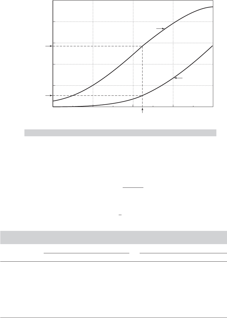
Figure 17.2 shows these two functions plotted over the range of GPA observed in the sample,
2.0 to 4.0. The marginal effect of PSI is the difference between the two functions, which ranges
from only about 0.06 at GPA = 2 to about 0.50 at GPA of 3.5. This effect shows that the
probability that a student’s grade will increase after exposure to PSI is far greater for students
with high GPAs than for those with low GPAs. At the sample mean of GPA of 3.117, the effect
of PSI on the probability is 0.465. The simple derivative calculation of (17-12) is given in Table
17.1; the estimate is 0.468. But, of course, this calculation does not show the wide range of
differences displayed in Figure 17.2.
Table 17.2 presents the estimated coefficients and marginal effects for the probit and
logit models in Table 17.2. In both cases, the asymptotic covariance matrix is computed
from the negative inverse of the actual Hessian of the log-likelihood. The standard errors for
the estimated marginal effect of PSI are computed using (17-24) and (17-25) since PSI is a
binary variable. In comparison, the simple derivatives produce estimates and standard errors
of (0.449, 0.181) for the logit model and (0.464, 0.188) for the probit model. These differ only
slightly from the results given in the table.
12
One might be tempted in this case to suggest an asymmetric distribution for the model, such as the Gumbel
distribution. However, the asymmetry in the model, to the extent that it is present at all, refers to the values
of ε, not to the observed sample of values of the dependent variable.
696
PART IV
✦
Cross Sections, Panel Data, and Microeconometrics
2.52.0
0
3.0
3.117
0.571
GPA
Prob(GRADE 1)
3.5 4.0
With PSI
Without PSI
1.0
0.8
0.6
0.4
0.2
0.106
FIGURE 17.2
Effect of
PSI
on Predicted Probabilities.
17.3.2.a Average Partial Effects
The preceding has emphasized computing the partial effects for the average individual in
the sample. Current practice has many applications based, instead, on “average partial
effects.” [See, e.g., Wooldridge (2002a).] The underlying logic is that the quantity of
interest is
APE = E
x
∂ E[y |x]
∂x
.
In practical terms, this suggests the computation
(
APE =
¯
ˆγ =
1
n
n
i=1
f (x
i
ˆ
β)
ˆ
β.
TABLE 17.2
Estimated Coefficients and Standard Errors (standard errors
in parentheses)
Logistic Probit
Variable Coefficient t Ratio Slope t Ratio Coefficient t Ratio Slope t Ratio
Constant −13.021 −2.641 — — −7.452 −2.931 — —
(4.931) (2.542)
GPA 2.826 2.238 0.534 2.252 1.626 2.343 0.533 2.294
(1.263) (0.237) (0.694) (0.232)
TUCE 0.095 0.672 0.018 0.685 0.052 0.617 0.017 0.626
(0.142) (0.026) (0.084) (0.027)
PSI 2.379 2.234 0.456 2.521 1.426 2.397 0.464 2.727
(1.065) (0.181) (0.595) (0.170)
log-likelihood −12.890 −12.819

CHAPTER 17
✦
Discrete Choice
697
This does raise two questions. Because the computation is (marginally) more burden-
some than the simple marginal effects at the means, one might wonder whether this
produces a noticeably different answer. That will depend on the data. Save for small
sample variation, the difference in these two results is likely to be small. Let
¯γ
k
= APE
k
=
1
n
n
i=1
∂Pr(y
i
= 1 |x
i
)
∂x
ik
=
1
n
n
i=1
F
(x
i
β)β
k
=
1
n
n
i=1
γ
k
(x
i
)
denote the computation of the average partial effect. We compute this at the MLE,
ˆ
β.
Now, expand this function in a second-order Taylor series around the point of sample
means,
¯
x, to obtain
¯γ
k
=
1
n
n
i=1
γ
k
(
¯
x) +
k
m=1
∂γ
k
(
¯
x)
∂ ¯x
m
(x
im
− ¯x
m
)
+
1
2
K
l=1
K
m=1
∂
2
γ
k
(
¯
x)
∂ ¯x
l
∂ ¯x
m
(x
il
− ¯x
l
)(x
im
− ¯x
m
)
+ ,
where is the remaining higher-order terms. The first of the three terms is the marginal
effect computed at the sample means. The second term is zero by construction. That
leaves the remainder plus an average of a term that is a function of the variances and
covariances of the data and the curvature of the probability function at the means. Little
can be said to characterize these two terms in any particular sample, but one might guess
they are likely to be small. We will examine an application in Example 17.4.
Based on the sample of observations on the partial effects, a natural estimator of
the variance of the partial effects would seem to be
ˆσ
2
γ,k
=
1
n − 1
n
i=1
ˆγ
k
(x
i
) −
¯
ˆγ
k
2
=
1
n − 1
n
i=1
PE
i,k
−
(
APE
k
2
.
See, for example, Contoyannis et al. (2004, p. 498), who report that they computed the
“sample standard deviation of the partial effects.” Since
(
AP E
k
=
¯
ˆγ
k
is the mean of a
sample, notwithstanding the following consideration, the preceding estimator should
be further divided by the sample size since we are computing the standard error of
the mean of a sample. This seems not to be the norm in the literature. This estimator
should not be viewed as an alternative to the delta method applied to the partial effects
evaluated at the means of the data, ˆγ (
¯
x). The delta method produces an estimator of
the asymptotic variance of an estimator of the population parameter, γ (μ
x
), that is, of
a function of
ˆ
β. The asymptotic covariance matrix computed using the delta method
for ˆγ (
¯
x) would be
ˆ
G(
¯
x)
ˆ
V
ˆ
G
(
¯
x) where
ˆ
G(
¯
x) is the matrix of partial derivatives and
ˆ
V
is the estimator of the asymptotic variance of
ˆ
β. This variance estimator converges to
zero because
ˆ
β converges to β and
¯
x converges to a vector of constants. The estimator
above does not converge to zero; it converges to the variance of the random variable
PE
i,k
.
The “asymptotic variance” of the partial effects estimator is intended to reflect the
variation of the parameter estimator,
ˆ
β, whereas the preceding estimator generates the
variation from the heterogeneity of the sample data while holding the parameter fixed

698
PART IV
✦
Cross Sections, Panel Data, and Microeconometrics
at
ˆ
β. For example, for a logit model,
ˆγ
k
(x
i
) =
ˆ
β
k
x
i
ˆ
β
1 −
x
i
ˆ
β
=
ˆ
β
k
ˆ
δ
i
,
and
ˆ
δ
i
is the same for all k. It follows that
ˆσ
2
γ,k
=
ˆ
β
2
k
1
n − 1
n
i=1
(
ˆ
δ
i
−
¯
ˆ
δ)
2
=
ˆ
β
2
k
s
2
ˆ
δ
.
A surprising consequence is that if one computes t ratios for the average partial effects
using ˆσ
2
γ,k
, the values will all equal the same 1/s
ˆ
δ
. This might signal that something is
amiss. (This is somewhat apparent in the Contoyannis et al. results on their page 498;
however, not enough digits were reported to see the effect clearly.)
A search for applications that use the delta method to estimate standard errors for
average partial effects in nonlinear models yields hundreds of occurrences. However,
we could not locate any that document in detail the precise formulas used. (One au-
thor, noting the complexity of computation, recommended bootstrapping instead.) A
complicated flaw with the sample variance estimator (notwithstanding all the preced-
ing) is that the estimator (whether scaled by 1/n or not) neglects the fact that all n
observations used to compute the estimated APE are correlated; they all use the same
estimator of β. The preceding estimator treats the estimates of PE
i
as if they were a
random sample. They would be if they were based on the true β. But the estimators
based on the same
ˆ
β are not uncorrelated. The delta method will account for the asymp-
totic (co)variation of the terms in the sum of functions of
ˆ
β. To use the delta method
to estimate the asymptotic standard errors for the average partial effects,
(
AP E
k
,we
should use
Est. Asy. Var
¯
ˆγ
=
1
n
2
Est. Asy. Var
n
i=1
ˆγ
i
=
1
n
2
n
i=1
n
j=1
Est. Asy. Cov
ˆγ
i
, ˆγ
j
=
1
n
2
n
i=1
n
j=1
G
i
(
ˆ
β)
ˆ
VG
j
(
ˆ
β)
=
1
n
n
i=1
G
i
(
ˆ
β)
ˆ
V
⎡
⎣
1
n
n
j=1
G
j
(
ˆ
β)
⎤
⎦
,
where
G
i
(
ˆ
β) =
∂ f
x
i
ˆ
β
ˆ
β
∂
ˆ
β
= f
x
i
ˆ
β
I + f
x
i
ˆ
β
ˆ
βx
i
.
This treats the APE as a point estimator of a population parameter—one that converges
in probability to what we assume is its population counterpart. But, it is conditioned on
the sample data; convergence is with respect to
ˆ
β. This looks like a formidable amount
of computation—Example 17.4 uses a sample of 27,326 observations, so it appears we
need a double sum of roughly 750 million terms. However, the computation is actually