Kopnin N.B. Theory of Nonequilibrium Superconductivity

Подождите немного. Документ загружается.

Here necessarily contains both retarded and advanced functions.

We now need to express the total self-energy in eqn (8.37) through the total

Green functions. Consider one of the jumps in the N-th order self-energy defined

by eqn (8.33); it is

(8.38)

Here . We took into account that the jump of the phonon

Green function at the cut l is nonzero only for the term with

The jump in the second line is taken at the cut where

. Putting where is real and

all

are still imaginary, we obtain

end p.155

Top

Oxford Scholarship Online: Theory of Nonequilibrium Supe... http://www.oxfordscholarship.com/oso/private/content/phy...

第7页共7页 2010-8-8 15:44

(8.39)

Performing the shift of the integration variable + =

, we have under the

integral

The jump in the third line of eqn (8.38) is taken at the cut where

Putting in the third line of eqn (8.38) we

get

(8.40)

The full expression for the jump becomes

(8.41)

Here we use the identity

Let us sum up all the jumps and collect all orders in N. We note that

Kopnin, Nikolai, Senior Scientist, Low Temperature Laboratory, Helsinki University of

Technology, and L.D. Landau Institute for Theoretical Physics, Moscow

Theory of Nonequilibrium Superconductivity

Print ISBN 9780198507888, 2001

pp. [156]-[160]

Oxford Scholarship Online: Theory of Nonequilibrium Supe... http://www.oxfordscholarship.com/oso/private/content/phy...

第1页共6页 2010-8-8 15:45

and

Finally, we arrive at the expression for the total self-energy

end p.156

(8.42)

Here the phonon functions D (P –P) depend on the momentum transfer while the

electron functions are of the form of

8.2.2 Order parameter

In the phonon model, the order parameter is defined as a part of the self-energy

(8.43)

(8.44)

The frequencies of the order of , i.e., in the range

where

is the

Debye frequency, are only important because the function F

vanishes for .

For such frequencies, one can put (D

+ D

)/2 = 1. As a result, is actually

independent of

and of the momentum p. It can be written simply in the form of

a BCS-type s-wave self-consistency equation

(8.45)

which coincides with eqn (8.28) if the square of the matrix element of the

PRINTED FROM OXFORD SCHOLARSHIP ONLINE (www.oxfordscholarship.com)

Oxford Scholarship Online: Theory of Nonequilibrium Supe... http://www.oxfordscholarship.com/oso/private/content/phy...

第2页共6页 2010-8-8 15:45

electron phonon interaction is replaced with |g|. We see that the phonon

model in the form of eqn (8.32) favors an s-wave pairing.

Separating

from the self-energy we obtain

where

and

and similarly for and .

end p.157

The diagonal components of the self-energy determine the renormalization of the

chemical potential

(8.46)

We can separate the contribution from the normal state by writing

. For the difference , the frequencies

~ are important. Therefore, we can neglect compared with

in the

phonon Green functions for this term. For the first term, the frequencies

only participate. For such frequencies, the Green functions coincide with their

values for the normal state with the accuracy (

)

; the difference can thus be

neglected in the weak coupling approximation. We have

(8.47)

where is the renormalization of the chemical potential in the normal state due

to the interaction with phonons. It only depends on the normal state properties

and can be disregarded. The second term in the r.h.s. is

where N is

the difference between the densities of electrons in the superconducting and in

the normal state according to eqn (8.30). In a good metal with a strong Coulomb

PRINTED FROM OXFORD SCHOLARSHIP ONLINE (www.oxfordscholarship.com)

Oxford Scholarship Online: Theory of Nonequilibrium Supe... http://www.oxfordscholarship.com/oso/private/content/phy...

第3页共6页 2010-8-8 15:45

interaction between electrons and ions of the crystalline lattice, the electronic

density is equal to the ion density, and does not change at a transition to the

superconducting state. If the Coulomb interaction is weak (or in case of

electrically neutral systems), the density change is

where

is the change in the chemical potential at the transition. In the weak

coupling approximation, where the electron: phonon interaction constant

, this term can also be neglected as compared to

itself. As a result, the diagonal term eqn (8.46) can be included into the

normal-state chemical potential and excluded from the consideration.

From now on we denote by

the new self-energy matrix which does not

contain the order parameter or the renormalization of the chemical potential

(8.48)

where and

. The self-energies defined by eqn (8.48) describe

inelastic relaxation processes and may be important for dynamical problems. In

the presence of impurities, the corresponding impurity self-energies should be

added to the phonon self-energies.

end p.158

FIG. 8.4. Diagram representation for the particle–particle self-energy.

As a result, the equations for the retarded and advanced Green functions now

have the form of eqns (8.19) with the operator [compare with eqn (8.3)]

PRINTED FROM OXFORD SCHOLARSHIP ONLINE (www.oxfordscholarship.com)

Oxford Scholarship Online: Theory of Nonequilibrium Supe... http://www.oxfordscholarship.com/oso/private/content/phy...

第4页共6页 2010-8-8 15:45

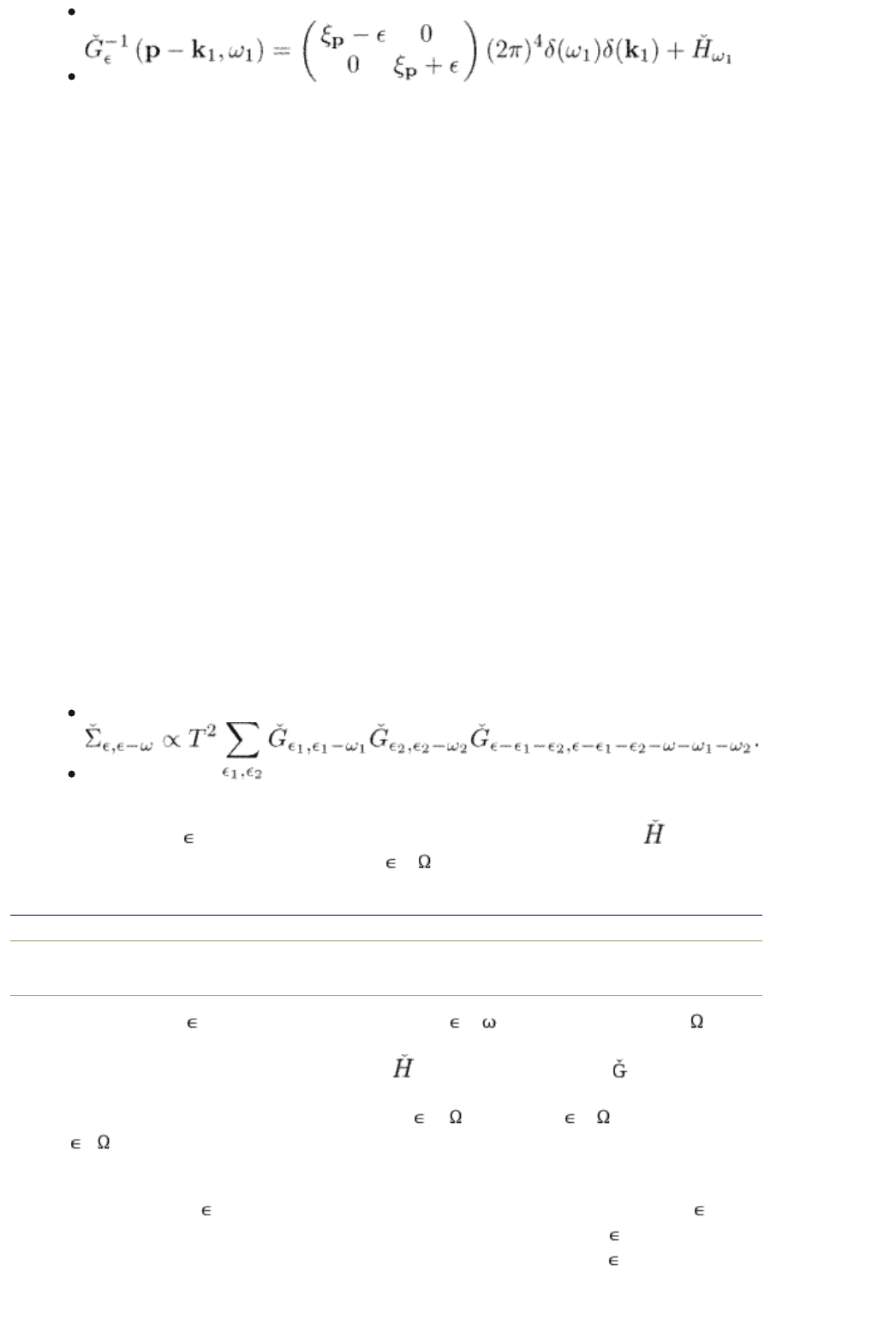
(8.49)

with the effective Hamiltonian determined by eqn (3.70). It now includes both

the electromagnetic potentials and the order parameter.

The equations for the anomalous and total Green functions are exactly the same

as eqns (8.55) and (8.61), The only difference is that the self-energy contains

the phonon contribution in the form of eqns (8.42), (8.48) in addition to the

impurity self-energies.

8.3 Particle–particle collisions

Electron–electron collisions in usual superconductors are not very important for

dynamic processes. This is in contrast with another Fermi superfluid,

He, where

the particle–particle collisions are not only responsible for kinetics of excitations

but also determine the pairing itself. In our discussion of superconductors,

however, we consider the pairing within the BCS model; particle–particle

collisions are only taken into account as long as they provide a relaxation

mechanism for excitations.

For degenerate Fermi system such as metals and

He, we can only consider

pairwise interactions of excitations which result in a self-energy shown in Fig.

8.4. The self-energy diagrams contain two vertexes connected by three particle

Green functions. In this section we do not consider the particular expressions for

the particle–particle self-energy. Instead, we shall only discuss the procedure of

analytical continuation for the self-energy of particle–particle interaction. The

particular expression for the relaxation parts of the self-energies are given in

Section 10.4.

We are interested in a sum in the form

(8.50)

Consider the contribution of the order N in the external field as a function of the

complex variable

for fixed imaginary frequencies of the field operator . It

has the singular lines determined by Im (

–

=0 which are located between

end p.159

the lowest line Im = 0 and the highest line Im ( – ) = 0. The frequencies

are combinations of the external field frequencies which now depend on the

particular distribution of the field vertices

between the functions in the sum

in eqn (8.50), i.e., between the internal lines of the diagram in Fig. 8.4. Consider

the term which has the singular lines at Im (

) = 0, Im ( –

) = 0, and

Im (

–

) = 0 and make the cuts along these lines. We now transform the

double sum over frequencies in eqn (8.50) into the double contour integral. We

shall make this transformation in two stages. On the first stage, the sum over

one frequency, say

, is transformed into the contour integral while keeping

as a fixed imaginary frequency. On the second stage, the sum over

transformed. During these transformations, the external frequency

and all field

frequencies are fixed at their imaginary values. The transformation of the

PRINTED FROM OXFORD SCHOLARSHIP ONLINE (www.oxfordscholarship.com)

Oxford Scholarship Online: Theory of Nonequilibrium Supe... http://www.oxfordscholarship.com/oso/private/content/phy...

第5页共6页 2010-8-8 15:45

particular term in eqn (8.50) gives

(8.51)

Here we omitted the second index at each for brevity.

Making now the analytical continuation of eqn (8.51) in

from the region Im (

– ) > 0 and, after that, in all field frequencies

from the upper half-plane, we

obtain

. Making the continuation in from the region Im < 0 and, after that,

in all field frequencies

from the upper half-plane, we obtain

. We are

interested in the relaxation part

–

. It is

(8.52)

Here

has the frequencies

–

etc., with

= –

–

, and

= –

Define the total self-energy according to eqn (8.37) as

end p.160

Top

Oxford Scholarship Online: Theory of Nonequilibrium Supe... http://www.oxfordscholarship.com/oso/private/content/phy...

第6页共6页 2010-8-8 15:45

(8.53)

We obtain

(8.54)

8.4 Transport-like equations and the conservation laws

One can derive kinetic-type equations for the anomalous and the total Green

functions. To do this, let us subtract eqn (8.26) from eqn (8.21). We obtain

(8.55)

The integration over internal variables is assumed for the expressions in the

square brackets

(8.56)

The internal frequency variables are shown explicitly in the last line of eqn.

(8.55). The momentum variables are not shown.

Equation (8.55) can also be written as

(8.57)

Kopnin, Nikolai, Senior Scientist, Low Temperature Laboratory, Helsinki University of

Technology, and L.D. Landau Institute for Theoretical Physics, Moscow

Theory of Nonequilibrium Superconductivity

Print ISBN 9780198507888, 2001

pp. [161]-[165]

Oxford Scholarship Online: Theory of Nonequilibrium Supe... http://www.oxfordscholarship.com/oso/private/content/phy...

第1页共6页 2010-8-8 15:46

where .

Subtracting eqn (8.27) from eqn (8.24) we find the equation for the total

function

end p.161

(8.58)

The “collision Integral” is

(8.59)

Equation (8.58) can be written as

(8.60)

because

p+k/2

–

p k/2

= v

k. It can also be represented in a more general form

(8.61)

Here

is shown in the coordinate representation. The momentum operator is p = – i

and E

(p) is the normal-state electronic spectrum. Equations (8.61, 8.25) or eqn

(8.55, 8.18) together with eqn (8.19) for the regular functions make the basis

for describing nonstationary properties of superconductors.

Equation (8.81) contains the conservation of particle number and the energy

conservation. To get the particle conservation

(8.62)

PRINTED FROM OXFORD SCHOLARSHIP ONLINE (www.oxfordscholarship.com)

Oxford Scholarship Online: Theory of Nonequilibrium Supe... http://www.oxfordscholarship.com/oso/private/content/phy...

第2页共6页 2010-8-8 15:46

we multiply eqn (8.61) with then take the trace and integrate it over

frequency d

/4 i and momentum d

p/ (2 )

. The terms of the form of *F

and

cancel out due to the self-consistency equation. One can also check that all

the collision integrals vanish under this operation (for example, the impurity

collision Integral already vanishes after integration over the momentum

directions).

To obtain the energy conservation, we multiply eqn (8.61) by

, take the trace

and Integrate it over frequency d

/4 i and momentum d

p/ (2 )

. We find

(8.63)

The Internal energy is

(8.64)

while the Internal energy current is

end p.162

(8.65)

We assume that the electronic system is in equilibrium with phonons. Otherwise,

there will be the additional energy source in the r.h.s, of eqn (8.63)

due to the interaction with phonons. The electron-electron collision integral

conserves the energy of interacting particles and thus drops out after integration

over d

with . The elastic impurity integral also conserves the energy; it already

vanishes after integration over the momentum directions.

The total energy

obeys the conservation equation

PRINTED FROM OXFORD SCHOLARSHIP ONLINE (www.oxfordscholarship.com)

Oxford Scholarship Online: Theory of Nonequilibrium Supe... http://www.oxfordscholarship.com/oso/private/content/phy...

第3页共6页 2010-8-8 15:46