Koren B., Vuik K. (Editors) Advanced Computational Methods in Science and Engineering
Подождите немного. Документ загружается.

Stefan Luding
adhesion (data not shown). This leads to a decrease of the stress-strain slope, then
the stress reaches a maximum and, for larger strain, turns into a softening failure
mode. As expected, the maximal stress is increasing with contact adhesion k
c
/k
2
.
The compressive strength is 6−7 times larger than the tensile strength, and a larger
adhesion force also allows for larger deformation before failure. The sample with
weakest adhesion, k
c
/k
2
= 1/2, shows tensile and compressive failure at strains
ε
xx
≈ −0.006 and
ε
xx
≈ 0.045, respectively.
Note that for tension, the post-peak behavior for the test with k
c
/k
2
= 20 is dif-
ferent from the other two cases, due to the strong particle-particle contact adhesion.
In this case, the tensile fracture occurs at the wall (except for a few particles that
remain in contact with the wall). This is in contrast to the other cases with smaller
bulk-adhesion, where the fracture occurs in the bulk, see Fig. 3.
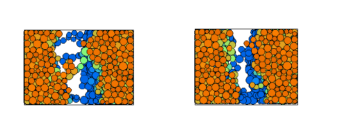
Fig. 3 Snapshots from tensile tests with k
c
/k
2
= 1/5 and 1, at horizontal strain of
ε
xx
≈ −0.8.
The color code denotes the distance from the viewer: blue, green, and red correspond to large,
moderate, and short distance.
3 Hard sphere molecular dynamics
In this section, the hard sphere model is introduced together with the event-driven
algorithm. A generalized model takes into account the finite contact duration of
realistic particles and, besides providing a physical parameter, saves computing time
because it avoids the “inelastic collapse”.
In the framework of the hard sphere model, particles are assumed to be perfectly
rigid and they follow an undisturbed motion until a collision occurs as described
below. Due to the rigidity of the interaction, the collisions occur instantaneously, so
that an event-driven simulation method [28, 51, 57, 56, 55] can be used. Note that
the ED method was only recently implemented in parallel [29, 57]; however, we
avoid to discuss this issue in detail.
468
From Particles to Continuum Theory
The instantaneous nature of hard sphere collisions is artificial, however, it is a
valid limit in many circumstances. Even though details of the contact- or collision
behavior of two particles are ignored, the hard sphere model is valid when binary
collisions dominate and multi-particle contacts are rare [44]. The lack of physical in-
formation in the model allows a much simpler treatment of collisions than described
in section 2 by just using a collision matrix based on momentum conservation and
energy loss rules. For the sake of simplicity, we restrict ourselves to smooth hard
spheres here. Collision rules for rough spheres are extensively discussed elsewhere,
see e.g. [47, 18], and references therein.
3.1 Smooth hard sphere collision model
Between collisions, hard spheres fly independently from each other. A change in
velocity – and thus a change in energy – can occur only at a collision. The stan-
dard interaction model for instantaneous collisions of identical particles with radius
a, and mass m, is used in the following. The post-collisional velocities v
′
of two
collision partners in their center of mass reference frame are given, in terms of the
pre-collisional velocities v, by
v
′
1,2
= v
1,2
∓(1 + r)v
n
/2 , (24)
with v
n
≡ [(v
1
−v
2
) ·n]n, the normal component of the relative velocity v
1
−v
2
,
parallel to n, the unit vector pointing along the line connecting the centers of the
colliding particles. If two particles collide, their velocities are changed according to
Eq. (24), with the change of the translational energy at a collision
∆
E = − m
12
(1 −
r
2
)v
2
n
/2, with dissipation for restitution coefficients r < 1.
3.2 Event-driven algorithm
Since we are interested in the behavior of granular particles, possibly evolving over
several decades in time, we use an event-driven (ED) method which discretizes the
sequence of events with a variable time step adapted to the problem. This is different
from classical DEM simulations, where the time step is usually fixed.
In the ED simulations, the particles follow an undisturbed translational motion
until an event occurs. An event is either the collision of two particles or the collision
of one particle with a boundary of a cell (in the linked-cell structure) [5]. The cells
have no effect on the particle motion here; they were solely introduced to accelerate
the search for future collision partners in the algorithm.
Simple ED algorithms update the whole system after each event, a method which
is straightforward, but inefficient for large numbers of particles. In Ref. [28] an ED
algorithm was introduced which updates only those two particles involved in the
469
Stefan Luding
last collision. Because this algorithm is “asynchronous” in so far that an event, i.e.
the next event, can occur anywhere in the system, it is so complicated to parallelize
it [57]. For the serial algorithm, a double buffering data structure is implemented,
which contains the ‘old’ status and the ‘new’ status, each consisting of: time of
event, positions, velocities, and event partners. When a collision occurs, the ‘old’
and ‘new’ status of the participating particles are exchanged. Thus, the former ‘new’
status becomes the actual ‘old’ one, while the former ‘old’ status becomes the ‘new’
one and is then free for the calculation and storage of possible future events. This
seemingly complicated exchange of information is carried out extremely simply and
fast by only exchanging the pointers to the ‘new’ and ‘old’ status respectively. Note
that the ‘old’ status of particle i has to be kept in memory, in order to update the time
of the next contact, t
i j
, of particle i with any other object j if the latter, independently,
changed its status due to a collision with yet another particle. During the simulation
such updates may be necessary several times so that the predicted ‘new’ status has
to be modified.
The minimum of all t
i j
is stored in the ‘new’ status of particle i, together with the
corresponding partner j. Depending on the implementation, positions and velocities
after the collision can also be calculated. This would be a waste of computer time,
since before the time t
i j
, the predicted partners i and j might be involved in several
collisions with other particles, so that we apply a delayed update scheme [28]. The
minimum times of event, i.e. the times, which indicate the next event for a certain
particle, are stored in an ordered heap tree, such that the next event is found at
the top of the heap with a computational effort of O(1); changing the position of
one particle in the tree from the top to a new position needs O(logN) operations.
The search for possible collision partners is accelerated by the use of a standard
linked-cell data structure and consumes O(1) of numerical resources per particle. In
total, this results in a numerical effort of O(N logN) for N particles. For a detailed
description of the algorithm see Ref. [28]. Using all these algorithmic tricks, we
are able to simulate about 10
5
particles within reasonable time on a low-end PC
[45], where the particle number is more limited by memory than by CPU power.
Parallelization, however, is a means to overcome the limits of one processor [57].
As a final remark concerning ED, one should note that the disadvantages con-
nected to the assumptions made that allow to use an event driven algorithm limit the
applicability of this method. Within their range of applicability, ED simulations are
typically much faster than DEM simulations, since the former account for a colli-
sion in one basic operation (collision matrix), whereas the latter require about one
hundred basic steps (integration time steps). Note that this statement is also true in
the dense regime. In the dilute regime, both methods give equivalent results, because
collisions are mostly binary [41]. When the system becomes denser, multi-particle
collisions can occur and the rigidity assumption within the ED hard sphere approach
becomes invalid.
The most striking difference between hard and soft spheres is the fact that soft
particles dissipate less energy when they are in contact with many others of their
kind. In the following chapter, the so called TC model is discussed as a means to
account for the contact duration t
c
in the hard sphere model.
470
From Particles to Continuum Theory
4 The link between ED and DEM via the TC model
In the ED method the contact duration is implicitly zero, matching well the corre-
sponding assumption of instantaneous contacts used for the kinetic theory [17, 22].
Due to this artificial simplification (which disregards the fact that a real contact takes
always finite time) ED algorithms run into problems when the time between events
t
n
gets too small: In dense systems with strong dissipation, t
n
may even tend towards
zero. As a consequence the so-called “inelastic collapse” can occur, i.e. the diver-
gence of the number of events per unit time. The problem of the inelastic collapse
[54] can be avoided using restitution coefficients dependent on the time elapsed
since the last event [51, 44]. For the contact that occurs at time t
i j
between particles
i and j, one uses r = 1 if at least one of the partners involved had a collision with
another particle later than t
i j
−t
c
. The time t
c
can be seen as a typical duration of a
contact, and allows for the definition of the dimensionless ratio
τ
c
= t
c
/t
n
. (25)
The effect of t
c
on the simulation results is negligible for large r and small t
c
; for a
more detailed discussion see [51, 45, 44].
In assemblies of soft particles, multi-particle contacts are possible and the in-
elastic collapse is avoided. The TC model can be seen as a means to allow for
multi-particle collisions in dense systems [43, 30, 51]. In the case of a homoge-
neous cooling system (HCS), one can explicitly compute the corrected cooling rate
(r.h.s.) in the energy balance equation
d
d
τ
E = −2I(E,t
c
) , (26)
with the dimensionless time
τ
= (2/3)At/t
E
(0) for 3D systems, scaled by A = (1−
r
2
)/4, and the collision rate t
−1
E
= (12/a)
ν
g(
ν
)
p
T/(
π
m), with T = 2K/(3N). In
these units, the energy dissipation rate I is a function of the dimensionless energy
E = K/K(0) with the kinetic energy K, and the cut-off time t
c
. In this representation,
the restitution coefficient is hidden in the rescaled time via A = A(r), so that inelastic
hard sphere simulations with different r scale on the same master-curve. When the
classical dissipation rate E
3/2
[17] is extracted from I, so that I(E,t
c
) = J(E,t
c
)E
3/2
,
one has the correction-function J → 1 for t
c
→ 0. The deviation from the classical
HCS is [44]:
J(E,t
c
) = exp(
Ψ
(x)) , (27)
with the series expansion
Ψ
(x) = −1.268x + 0.01682x
2
−0.0005783x
3
+ O(x
4
) in
the collision integral, with x =
√
π
t
c
t
−1
E
(0)
√
E =
√
πτ
c
(0)
√
E =
√
πτ
c
[44]. This is
close to the result
Ψ
LM
= −2x/
√
π
, proposed by Luding and McNamara, based on
probabilistic mean-field arguments [51]
3
.
Given the differential equation (26) and the correction due to multi-particle con-
tacts from Eq. (27), it is possible to obtain the solution numerically, and to compare
3
Ψ
LM
thus neglects non-linear terms and underestimates the linear part
471
Stefan Luding
1
10
100
1000
0.01 0.1 1 10 100 1000
E/E
τ
τ
τ
c
=2.4
τ
c
=1.2
τ
c
=0.60
τ
c
=0.24
τ
c
=1.2 10
-2
τ
c
=1.2 10
-4
0.98
1
1.02
1.04
1.06
1.08
1.1
1.12
1.14
1.16
0.01 0.1 1 10 100
E/E
τ
τ
t
c
=10
-2
t
c
=5.10
-3
t
c
=10
-3
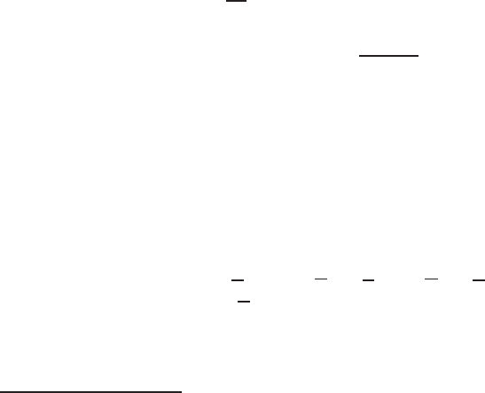
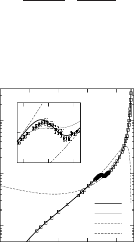
Fig. 4 (Left) Deviation from the HCS, i.e. rescaled energy E/E
τ
, where E
τ
is the classical solution
E
τ
= (1 +
τ
)
−2
. The data are plotted against
τ
for simulations with different
τ
c
(0) = t
c
/t
E
(0) as
given in the inset, with r = 0.99, and N = 8000. Symbols are ED simulation results, the solid
line results from the third order correction. (Right) E/E
τ
plotted against
τ
for simulations with
r = 0.99, and N = 2197. Solid symbols are ED simulations, open symbols are DEM (soft particle
simulations) with three different t
c
as given in the inset.
it to the classical E
τ
= (1 +
τ
)
−2
solution. Simulation results are compared to the
theory in Fig. 4 (left). The agreement between simulations and theory is almost
perfect in the examined range of t
c
-values, only when deviations from homogene-
ity are evidenced one expects disagreement between simulation and theory. The
fixed cut-off time t
c
has no effect when the time between collisions is very large
t
E
≫ t
c
, but strongly reduces dissipation when the collisions occur with high fre-
quency t
−1
E
>
∼ t
−1
c
. Thus, in the homogeneous cooling state, there is a strong effect
initially, and if t
c
is large, but the long time behavior tends towards the classical
decay E → E
τ
∝
τ
−2
.
The final check if the ED results obtained using the TC model are reasonable is
to compare them to DEM simulations, see Fig. 4 (right). Open and solid symbols
correspond to soft and hard sphere simulations respectively. The qualitative behav-
ior (the deviation from the classical HCS solution) is identical: The energy decay is
delayed due to multi-particle collisions, but later the classical solution is recovered.
A quantitative comparison shows that the deviation of E from E
τ
is larger for ED
than for DEM, given that the same t
c
is used. This weaker dissipation can be under-
stood from the strict rule used for ED: Dissipation is inactive if any particle had a
contact already. The disagreement between ED and DEM is systematic and should
disappear if an about 30% smaller t
c
value is used for ED. The disagreement is also
plausible, since the TC model disregards all dissipation for multi-particle contacts,
while the soft particles still dissipate energy - even though much less - in the case of
multi-particle contacts.
The above simulations show that the TC model is in fact a “trick” to make hard
particles soft and thus connecting between the two types of simulation models: soft
and hard. The only change made to traditional ED involves a reduced dissipation for
(rapid) multi-particle contacts.
472

From Particles to Continuum Theory
5 The stress in particle simulations
The stress tensor is a macroscopic quantity that can be obtained by measurement
of forces per area, or via a so-called micro-macro homogenization procedure. Both
methods will be discussed below. During derivation, it also turns out that stress has
two contributions, the first is the “static stress” due to particle contacts, a potential
energy density, the second is the “dynamics stress” due to momentum flux, like
in the ideal gas, a kinetic energy density. For the sake of simplicity, we restrict
ourselves to the case of smooth spheres here.
5.1 Dynamic stress
For dynamic systems, one has momentum transport via flux of the particles. This
simplest contribution to the stress tensor is the standard stress in an ideal gas, where
the atoms (mass points) move with a certain fluctuation velocity v
i
. The kinetic
energy E =
∑
N
i=1
mv
2
i
/2 due to the fluctuation velocity v
i
can be used to define the
temperature of the gas k
B
T = 2E/(DN), with the dimension D and the particle
number N. Given a number density n = N/V, the stress in the ideal gas is then
isotropic and thus quantified by the pressure p = nk
B
T; note that we will disregard
k
B
in the following. In the general case, the dynamic stress is
σ
= (1/V)
∑
i
m
i
v
i
⊗v
i
,
with the dyadic tensor product denoted by ‘⊗’, and the pressure p = tr
σ
/D = nT is
the kinetic energy density.
The additional contribution to the stress is due to collisions and contacts and will
be derived from the principle of virtual displacement for soft interaction potentials
below, and then be modified for hard sphere systems.
5.2 Static stress from virtual displacements
From the centers of mass r
1
and r
2
of two particles, we define the so-called branch
vector l = r
1
−r
2
, with the reference distance l = |l| = 2a at contact, and the cor-
responding unit vector n = l/l. The deformation in the normal direction, relative
to the reference configuration, is defined as
δ
= 2an −l. A virtual change of the
deformation is then
∂δ
=
δ
′
−
δ
≈
∂
l =
ε
·l , (28)
where the prime denotes the deformation after the virtual displacement described
by the tensor
ε
. The corresponding potential energy density due to the contacts of
one pair of particles is u = k
δ
2
/(2V), expanded to second order in
δ
, leading to the
virtual change
∂
u =
k
V
δ
·
∂δ
+
1
2
(
∂δ
)
2
≈
k
V
δ
·
∂
l
n
, (29)
473
Stefan Luding
where k is the spring stiffness (the prefactor of the quadratic term in the series ex-
pansion of the interaction potential), V is the averaging volume, and
∂
l
n
= n(n·
ε
·l)
is the normal component of
∂
l. Note that
∂
u depends only on the normal component
of
∂δ
due to the scalar product with
δ
, which is parallel to n.
From the potential energy density, we obtain the stress from a virtual deformation
by differentiation with respect to the deformation tensor components
σ
=
∂
u
∂ε
=
k
V
δ
⊗l =
1
V
f ⊗l , (30)
where f = k
δ
is the force acting at the contact, and the dyadic product ⊗ of two
vectors leads to a tensor of rank two.
5.3 Stress for soft and hard spheres
Combining the dynamic and the static contributions to the stress tensor [49], one
has for smooth, soft spheres:
σ
=
1
V
"
∑
i
m
i
v
i
⊗v
i
−
∑
c∈V
f
c
⊗l
c
#
, (31)
where the right sum runs over all contacts c in the averaging volume V. Replacing
the force vector by momentum change per unit time, one obtains for hard spheres:
σ
=
1
V
"
∑
i
m
i
v
i
⊗v
i
−
1
∆
t
∑
n
∑
j
p
j
⊗l
j
#
, (32)
where p
j
and l
j
are the momentum change and the center-contact vector of particle
j at collision n, respectively. The sum in the left term runs over all particles i, the
first sum in the right term runs over all collisions n occurring in the averaging time
∆
t, and the second sum in the right term concerns the collision partners of collision
n [51].
Exemplary stress computations from DEM and ED simulations are presented in the
following section.
6 2D simulation results
Stress computations from two dimensional DEM and ED simulations are presented
in the following subsections. First, a global equation of state, valid for all densities,
is proposed based on ED simulations, and second, the stress tensor from a slow,
474
From Particles to Continuum Theory
quasi-static deformation is computed from DEM simulations with frictional parti-
cles.
6.1 The equation of state from ED
The mean pressure in two dimensions is p = (
σ
1
+
σ
2
)/2, with the eigenvalues
σ
1
and
σ
2
of the stress tensor [48, 49, 32]. The 2D dimensionless, reduced pres-
sure P = p/(nT ) −1 = pV/E −1 contains only the collisional contribution and the
simulations agree nicely with the theoretical prediction P
2
= 2
ν
g
2
(
ν
) for elastic
systems, with the pair-correlation function g
2
(
ν
) = (1 −7
ν
/16)/(1 −
ν
)
2
, and the
volume fraction
ν
= N
π
a
2
/V, see Fig. 5. A better pair-correlation function is
g
4
(
ν
) =
1 −7
ν
/16
(1 −
ν
)
2
−
ν
3
/16
8(1 −
ν
)
4
, (33)
which defines the non-dimensional collisional stress P
4
= 2
ν
g
4
(
ν
). For a system
with homogeneous temperature, as a remark, the collision rate is proportional to the
dimensionless pressure t
−1
n
∝ P.
1
10
100
0 0.2 0.4 0.6 0.8
P
ν
Q
Q
0
P
4
P
dense
8
9
10
0.68 0.7 0.72
Fig. 5 The dashed lines are P
4
and P
dense
as functions of the volume fraction
ν
, and the symbols
are simulation data, with standard deviations as given by the error bars in the inset. The thick solid
line is Q, the corrected global equation of state from Eq. (34), and the thin solid line is Q
0
without
empirical corrections.
When plotting P against
ν
with a logarithmic vertical axis, in Fig. 5, the sim-
ulation results can almost not be distinguished from P
2
for
ν
< 0.65, but P
4
leads
475

Stefan Luding
to better agreement up to
ν
= 0.67. Crystallization is evidenced at the point of the
liquid-solid transition
ν
c
≈0.7, and the data clearly deviate from P
4
. The pressure is
strongly reduced due to the increase of free volume caused by ordering. Eventually,
the data diverge at the maximum packing fraction
ν
max
=
π
/(2
√
3) for a perfect
triangular array.
For high densities, one can compute from free-volume models, the reduced pres-
sure P
fv
= 2
ν
max
/(
ν
max
−
ν
). Slightly different functional forms do not lead to
much better agreement [32]. Based on the numerical data, we propose the corrected
high density pressure P
dense
= P
fv
h(
ν
max
−
ν
) −1, with the empirical fit function
h(x) = 1 + c
1
x+ c
3
x
3
, and c
1
= −0.04 and c
3
= 3.25, in perfect agreement with the
simulation results for
ν
≥ 0.73.
Since, to our knowledge, there is no conclusive theory available to combine the
disordered and the ordered regime [23], we propose a global equation of state
Q = P
4
+ m(
ν
)[P
dense
−P
4
] , (34)
with an empirical merging function m(
ν
) = [1 + exp(−(
ν
−
ν
c
)/m
0
)]
−1
, which se-
lects P
4
for
ν
≪
ν
c
and P
dense
for
ν
≫
ν
c
, with the transition density
ν
c
and the
width of the transition m
0
. In Fig. 5, the fit parameters
ν
c
= 0.702 and m
0
≈0.0062
lead to qualitative and quantitative agreement between Q (thick line) and the sim-
ulation results (symbols). However, a simpler version Q
0
= P
2
+ m(
ν
)[P
fv
−P
2
],
(thin line) without empirical corrections leads already to reasonable agreement when
ν
c
= 0.698 and m
0
= 0.0125 are used. In the transition region, this function Q
0
has
no negative slope but is continuous and differentiable, so that it allows for an easy
and compact numerical integration of P. We selected the parameters for Q
0
as a
compromise between the quality of the fit on the one hand and the simplicity and
treatability of the function on the other hand.
As an application of the global equation of state, the density profile of a dense
granular gas in the gravitational field has been computed for monodisperse [49] and
bidisperse situations [48, 32]. In the latter case, however, segregation was observed
and the mixture theory could not be applied. The equation of state and also other
transport properties are extensively discussed in Refs. [4, 1, 3, 2] for 2D, bi-disperse
systems.
6.2 Quasi-static DEM simulations
In contrast to the dynamic, collisional situation discussed in the previous section, a
quasi-static situation, with all particles almost at rest most of the time, is discussed
in the following.
476

From Particles to Continuum Theory
6.2.1 Model parameters
The systems examined in the following contain N = 1950 particles with radii a
i
ran-
domly drawn from a homogeneous distribution with minimum a
min
= 0.510
−3
m
and maximum a
max
= 1.510
−3
m. The masses m
i
= (4/3)
ρπ
a
3
i
, with the density
ρ
= 2.010
3
kg m
−3
, are computed as if the particles were spheres. This is an arti-
ficial choice and introduces some dispersity in mass in addition to the dispersity in
size. Since we are mainly concerned about slow deformation and equilibrium situ-
ations, the choice for the calculation of mass should not matter. The total mass of
the particles in the system is thus M ≈ 0.02 kg with the typical reduced mass of a
pair of particles with mean radius, m
12
≈ 0.4210
−5
kg. If not explicitly mentioned,
the material parameters are k
2
= 10
5
N m
−1
and
γ
0
= 0.1 kg s
−1
. The other spring-
constants k
1
and k
c
will be defined in units of k
2
. In order to switch on adhesion,
k
1
< k
2
and k
c
> 0 is used; if not mentioned explicitly, k
1
= k
2
/2 is used, and k
2
is
constant, independent of the maximum overlap previously achieved.
Using the parameters k
1
= k
2
and k
c
= 0 in Eq. (4) leads to a typical contact du-
ration (half-period): t
c
≈2.0310
−5
s for
γ
0
= 0, t
c
≈2.0410
−5
s for
γ
0
= 0.1 kg s
−1
,
and t
c
≈ 2.2110
−5
s for
γ
0
= 0.5 kg s
−1
for a collision. Accordingly, an integration
time-step of t
DEM
= 510
−7
s is used, in order to allow for a ‘safe’ integration of con-
tacts involving smaller particles. Large values of k
c
lead to strong adhesive forces,
so that also more energy can be dissipated in one collision. The typical response
time of the particle pairs, however, is not affected so that the numerical integration
works well from a stability and accuracy point of view.
6.2.2 Boundary conditions
The experiment chosen is the bi-axial box set-up, see Fig. 6, where the left and
bottom walls are fixed, and stress- or strain-controlled deformation is applied. In the
first case a wall is subject to a predefined pressure, in the second case, the wall is sub-
ject to a pre-defined strain. In a typical ‘experiment’, the top wall is strain controlled
and slowly shifted downwards while the right wall moves stress controlled, depen-
dent on the forces exerted on it by the material in the box. The strain-controlled
position of the top wall as function of time t is here
z(t) = z
f
+
z
0
−z
f
2
(1 + cos
ω
t) , with
ε
zz
= 1 −
z
z
0
, (35)
where the initial and the final positions z
0
and z
f
can be specified together with the
rate of deformation
ω
= 2
π
f so that after a half-period T/2 = 1/(2 f ) the extremal
deformation is reached. With other words, the cosine is active for 0 ≤
ω
t ≤
π
. For
larger times, the top-wall is fixed and the system can relax indefinitely. The cosine
function is chosen in order to allow for a smooth start-up and finish of the motion
so that shocks and inertia effects are reduced, however, the shape of the function is
arbitrary as long as it is smooth.
The stress-controlled motion of the side-wall is described by
477