Mark James E. (ed.). Physical Properties of Polymers Handbook

Подождите немного. Документ загружается.

g-phase, at the expense of the commonly encountered

a-phase.

For further information on current thinking and theoret-

ical approaches to crystallization, the reader is referred to

recent reviews by Phillips [32,33].

39.1.2 Case Study Using Isotactic Polypropylene

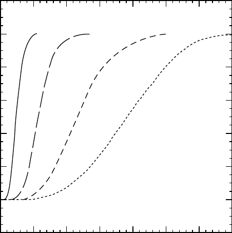
Figure 39.4 shows several chart recorded bulk crystalliza-

tion traces as a function of temperatures for isotactic poly-

propylene (iPP, M

¼ 257,000). Avrami’s analysis takes

the lower values of each plot; i.e., before impingement.

The half-time is the point where half of the intensity is

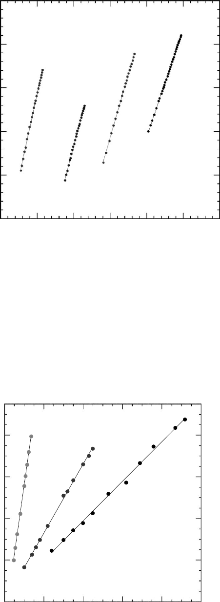
reached. Figure 39.5 presents Avrami’s analysis for differ-

ent crystallization temperatures, where it can be seen that all

plots have similar slope, n, and different intercepts, k,in

this case.

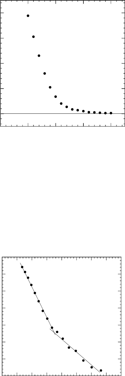
Examples of the change in spherulite radius with time for

selected temperatures are shown in Fig. 39.6, where it

can be seen that linear growth rates result. Plots of growth

rate versus temperature for iPP can be seen in Fig. 39.7.

When the data are analyzed using the Hoffman–Lauritzen

equation, Fig. 39.8, it is seen that iPP shows the Regime

II–Regime III transition, previously identified by several

groups of workers [7–10]. In these analyses the values of

and U



were 186.1 8 C and 1,500 cal/mol, respectively.

The effects of different values of the thermodynamic

variables on the analyses and on the regime transition tem-

perature have been explored. Variation in T

has the great-

est effect on the shape of the secondary nucleation plot, but

does not significantly alter the regime transition tempera-

ture. A small change of the values of U



and T

simply

causes the curve to move up or down without changing its

shape.

The Regime II–III transition is envisioned as the point at

which the rate of surface spreading becomes less than

the rate of secondary nucleation. Surface spreading, for

an adjacent reentry system, is essentially a reeling-in pro-

cess dependent on the reptational ability of the polymer

chain.

The slopes of the secondary nucleation plots can be used

to estimate the fold surface free energies of the two poly-

mers. In order for these calculations to be carried out it

is necessary to have estimates of the parameters which

appear within Eq. 39.5. The equilibrium melting point

has to be determined in separate experimentation (see

Chapter 11).

The values of ss

can be determined from the slope of

the lines. Regime II and regime III give ss

¼ 562 and

678 erg

=cm

, respectively. In order to proceed further it is

necessary to estimate s independently. One way to do this is

to use the Hoffman modification of the Thomas–Stavely

relation [24].

s ¼ 0:1Dh

ﬃﬃﬃﬃﬃﬃﬃﬃﬃ

: (39:6)

Values of s have been calculated as 11:5 erg=cm

for iPP.

Substitution of these values into the determined values of

−0.2

0.2

0.4

0.6

0.8

1.2

0 5 10 15 20 25 30 35

Light intensity

Time (min)

124 °C 126 °C 132 °C 134 °C

FIGURE 39.4. Isothermal bulk crystallization traces as a function of temperature.

CRYSTALLIZATION KINETICS OF POLYMERS / 629

results in values of s

for regime II and regime III of

48.9 and 59:0 erg=cm

, respectively.

The work done by the chain (q) to form a fold can be

easily calculated from the following equation, when the fold

surface energy is known.

q ¼ 2a

(39:7)

39.1.3 Tabulation of Data

In the tabulation, data are presented mainly for common

homopolymers. When available, molecular weights are

also given, but no major attempt has been made to present

molecular weight dependencies. Additionally, a few illus-

trations of specific copolymers have been included as

examples of copolymer behavior.

−4

−3

−2

−1

1234567

ln(− ln(1−

I))

ln(t )

126 °C

132

°C

136

°C

142

°C

FIGURE 39.5. Avrami analyses for different crystallization temperatures.

0 20406080100

Radius (µm)

Time (min)

130

°C

136

°C

140

°C

FIGURE 39.6. Spherulitic growth of iPP as a function of time for different isothermal crystallization temperatures.

630 / CHAPTER 39

It should be recognized that Avrami data can vary greatly

with the presence of additives, especially nucleating agents.

In Table 39.2 data are presented from bulk crystallization

studies of common polymers.

In Table 39.3 data are presented from linear growth

rate studies of polymers that are commonly encountered

in significant basic studies or that are of commercial signifi-

cance. In addition to the values of the characteristic param-

eters obtained from the analyses, we have added the value of

other constants such as equilibrium melting points and heats

of fusion which are essential to the analyses.

110 120 130 140 150

G (µm/min)

(°C)

FIGURE 39.7. Growth rates of iPP versus crystallization temperature.

3.5 4 4.5 5 5.5 6 6.5 7 7.5

∆

= 138.0 ˚C

ln(G ) + U

*/R (T

−T

∞

)

(10

)/(T

−

∆Tf )

FIGURE 39.8. Secondary nucleation analyses of iPP using T

of 186.1 8C.

CRYSTALLIZATION KINETICS OF POLYMERS / 631

TABLE 39.2. Avrami coefficients.

Polymer

(kg/mol)

(8C)

1=2

(s) n

n

) Remarks Ref.

194.8 43 2.5 DSC [34]

16.0 29.0 197.4 75 2.9

200.4 110 3.6

202.6 200 4.0

Nylon 6

205.5 350 4.8

140 10 3 DLM [35]

24.7 160 15 3

180 70 3

200 950 3

Poly (amide)

( min

n

) DSC [36]

165 46.2 2.21 1:34  10

4

Nylon 10 12

167 68.4 1.97 1:54  10

4

169 144.6 1.91 5:37  10

5

171 241.8 1.91 1:90  10

5

173 450 2.08 1:86  10

6

( min

n

) DSC [37]

164 10.3 1.6 1:23  10

Nylon 11

166 16.5 2.1 1:0  10

168 23.1 2.4 6.92

170 43.8 2.7 1.62

172 85.8 3.2 2:2  10

1

( min

n

) DSC [38]

Nylon 12 12

160 34.8 2.03 2.12

164 63.6 1.67 6:2  10

1

168 119.4 1.68 2:2 10

1

170 231.6 1.64 8:0  10

2

70 60 DLM [39]

Poly (butene-1) PB-1 73 750 80 96

90 456

95 1572

40 4.5 3.46 DSC [40]

Poly (e- PCL 43.6 48 45 17.9 3.35

caprolactone) 47 45.8 2.48

49 97.6 2.66

Poly (chlorotri- 180 180 3 Dilatometry [41]

fluoroethylene) PCTFE 186 480 3

191 1500 3

196 4200 3

124 165 2.35 DSC [42]

125 338 2.29

126 750 2.05

Polyethylene

HDPE

127 1920 2.24

117 0.24 3.1 DLM [43]

12.7 42.3 119 0.67 2.9

121 4.00 3.0

123 20.00 2.7

Polyethylene XLPE cross- 4.5 8.7 119 3.5 2.7 [43]

link 255 avg 120 1.25 2.2

units 123 3.5

124 3.6

632 / CHAPTER 39

TABLE 39.2. Continued.

Polymer

(kg/mol)

(8C)

1=2

(s) n

n

) Remarks Ref.

175.2 4.7 1:6  10

8

DSC [44]

Poly (aryl-ether– PEEK 182.3 5.7 4:7  10

10

ether–ketone) 188.8 5.1 1:8  10

7

( min

n

)

180 2.36 1:02  10

2

DSC [45]

19 40 190 2.30 7:43  10

3

200 2.43 2:04  10

3

Poly (ethylene- PET 210 2.37 2:63  10

4

terephthalate) 190 63 1.83 DSC [46]

195 86 1.76

200 133 1.77

210 190 1.76

185 150 2.61 1:52  10

6

DSC [47]

Poly (propylene- PPT 36.3 78.4 190 250 2.59 4:03  10

7

terephthalate) 195 500 2.61 6:51  10

8

200 1,000 2.48 2:42  10

8

180 50 75 2.47 5:61  10

5

DSC [47]

Poly (butylene- PBT 36.6 77.4 185 150 2.49 1:65  10

5

terephthalate) 190 340 2.48 2:74  10

6

195 2.55 2:79  10

7

2.3 ( min

n

)

170 2.6 3.0 7.9

43 180 2.9 3.2 3.67

190 0.43 DSC [48]

200 9:96  10

3

Poly (trimethylene

ter-ephthalate)

PTT 210 5:75  10

6

( min

n

)

21.05 46.3 202 174 2.81 33:7  10

3

206 279 2.72 10:8 10

3

DSC [49]

210 592 2.84 1:0  10

3

38 23,400 [50]

33 1,440

cis-PIP 22 9,000 [51]

16 12,000

11 19,800 [52]

Poly (isoprene) 5 55,200

35 768

40 1,260

trans-PIP 45 6,780

51 31,800

57 2,91,000

40.1 1.9 0:18  10

DSC [53]

Poly (oxyethylene) POE

9.0 9.6 43.4 2.0 6:8  10

1

48.4 2.3 2:6  10

2

49.6 2.1 8:3  10

4

55 612 1.8 DSC [54]

20 56 1,200 1.9

57 1,476 2.0

58 4,884 2.1

59 6,900 2.5

CRYSTALLIZATION KINETICS OF POLYMERS / 633

TABLE 39.2. Continued.

Polymer

(kg/mol)

(8C)

1=2

(s) n

n

) Remarks Ref.

40.3 1,650 3.0 DLM [55]

Poly POP 300 42.8 2,520 3.1

(oxypropylene) 45.5 3,540 3.3

47.5 8,580 3.0

49.7 12,600 3.1

230 160 1.84 DSC [56]

Poly (phenylene PPS 235 195 2.14

sulfide) 240 370 2.12

245 580 2.08

130 430 3.11 1:29 10

3

DLM [57]

58.0 151 132 650 2.61 7:59 10

4

136 3,200 2.84 1:41  10

4

142 13,500 2.91 1:15  10

5

Polypropylene iPP 130 780 3.1 DLM [58]

447 133 2,220 2.9

134 2,820 2.9

137 6,600 2.9

60 100 2.68 1:06  10

DSC [59]

76.2 165 70 118 2.68 6.66

80 210 3.07 8:82  10

1

90 684 2.96 3:11  10

2

Polypropylene sPP 95 1,698 2.41 1:33  10

2

75 56 2.44 4:72  10

DSC [59]

52.3 195 80 100 2.33 1:24  10

90 439 2.40 3:43  10

1

95 1,294 2.32 3:40  10

2

80 32,400 2.01 1: 05  10

2

[60]

Selenium 100 3,600 1.68 0:61  10

120 720 3.28 1:20  10

dynamic

140 280 3.68 3:60  10

density

160 105 4.00 2:60  10

148 163.2 2.67 4:16  10

2

Poly POM 149 316.2 2.59 9:48  10

2

DSC [61]

(oxymethylene) 150 607.8 2.36 3:17  10

3

151 1,141.2 2.98 1:08  10

4

296 0.057 0.96 1:21  10

Poly (tetrafluoro- PTFE 304 0.116 1.01 5.97 DSC [62]

ethylene) 312 0.332 1.006 2.09

315 0.301 0.87 1.97

236 16.73 1.9 4:76  10

Polystyrene sPS 91.6 220 239 50.21 1.4 5:29  10

DSC [63]

242 96.33 1.3 2:26  10

244 135.14 1.1 1:60  10

( min

n

)

192 2,400 2.73 3:05  10

7

Poly (arylene-ether– 34 200 4,800 2.8 4:13  10

8

ether–phenylsulfide) 211 30,000 2.8 9:23  10

9

DSC [64]

218 60,000 2.73 2:27  10

9

226 600,000 2.73 1:69  10

10

634 / CHAPTER 39

TABLE 39.2. Continued.

Polymer

(kg/mol)

(8C)

1=2

(s) n

n

) Remarks Ref.

( min

n

)

Poly (arylene- 19.1 279 5,400 1.7 2:75  10

5

ether–ether– 285 30,000 1.7 1:01  10

5

DSC [64]

biphenylsulfide) 290 48,000 1.9 1:37  10

6

110 19.2 2.52 6:25  10

4

Poly 120 91.8 3.06 0:8  10

6

(ester–amide) 130 2,124 2.71 7:4  10

10

DSC [65]

135 3,180 2.20 1:31  10

8

29 18 3.1 8:9  10

5

Poly (butylene PBA 7.3 35 42 2.6 4:2  10

5

adipate) 40 180 3.0 1:2  10

7

DSC [66]

43 486 3.1 3:3  10

9

45 1,156 3.1 45  10

10

70.2 1272 2.9 6:9  10

10

Poly (butylene PBIP 13 80.2 630 2.9 5:3  10

9

DSC [66]

isophthalate) 90.2 498 2.8 1:9  10

8

100.2 456 3.0 7:3  10

9

109.7 672 3.0 2:3  10

9

118.7 1,068 3.1 2:8  10

10

123.7 1,590 2.9 3:6  10

10

( min

n

)

180 408 2.4 7:1  10

3

Poly (ethylene PEN 190 270 2.9 8:6  10

3

(DSC) [67]

naphthalate) 200 174 2.7 3:8  10

2

210 186 3.2 2:0  10

2

220 204 3.1 1:6  10

2

230 384 2.3 9:2  10

3

240 1,507 2.39

Polyimide* 260 600 2.37 (DSC) [68]

280 444 2.3

300 600 2.32

320 1,197

( min

n

)

147 192 2.9 1:88  10

2

Poly (vinylidene PVDF 170 151 720 2.9 3:12  10

4

(DSC) [69]

fluoride) 153 960 3.1 1:28  10

4

155 1,800 2.9 1:83  10

5

( min

n

)

176 97.8 3.2 1:45  10

1

1, 2-Syndiotactic 1, 2-sPB 177 126 2.8 8:68  10

2

(DSC) [70]

Polybutadiene 178 169.2 3.0 3:09  10

2

179 223.8 2.8 1:74  10

2

180 358.2 2.9 3:9  10

3

*Polyimide synthesized from 3, 3’,4,4’-benzophenonetetracarboxylic dianhydride (BTDA) and 2, 2-dimethyl-1, 3-(4-amino-

phenoxy) propane (DMDA).

CRYSTALLIZATION KINETICS OF POLYMERS / 635

TABLE 39.3.

Growth kinetics coefficients.

Polymer

(kg=mol)

kg=mol

(



(



(J=g)

Growth

face

)



(cal=mol)

Regime

(



(cm=s)

=10

)

(erg

=cm

)

(erg=cm

)

(kcal

=mol)

Ref.

Poly(amide)

Nylon 6

30 232.0

4.78 3.70 1,430

0:65 

1.74

118 6.0 [71]

24.7

10 230 10.8

(kcal/mol)

4.78 3.70 1,840

1:05  10

6.70 8.0 65

[72]

Nylon 66

45.0 272 200.8

4.76 3.70 167

1:55  10

1.02 8.0 40

[72]

Nylon 11

41.96 202.8 217

(J=cm

)

(100) 5.4 4.44 1,500 II

1.66 10.6 110.6 7.61 [37]

Poly(butene-1)

PB-1

54:2 127.8

1,500

0:25  10

0.79

[71]

Poly(e-

caprolactone)

PCL

26 40

60 70.3 163

(J=cm

)

(110) 4.52 4.12 1,500

0.80 6.7 94.7 5.06 [73]

43.6 48

63 74 148

(J=cm

)

(110) 4.50 4.10 1,500

6:03  10

0.91 6.1 106

[40]

Poly(chlorotrifluoro

ethylene)

PCTFE

52.0 224.0

6.50 5.60 4,000

6:50  10

1.72

53 5.6 [71]

400

52 224 91

(J=cm

)

6.50 5.60

0:17  10

0.17 5.2 36 3.8 [74]

Polyethylene

PE single

crystals

30 63

42 114 280

(J=cm

)

(110) 4.15 4.55 1,500 I

2.11 13.7 93.4 5.1 [3]

30.6

42:2 144.6 280

(J=cm

)

4.55 4.15 1,500 I

4:40  10

2.16 14.1 90.4 5.0 [71]

II 127 2

:24 

1.15 14.1 97.8

20 141 280

(J=

)

(110) 4.45 4.11

16:00  10

1.24 12.2 49 2.6 [74]

HDPE

13.0 18.1

40:0 144.5 288.7

1,500 I

1:45 

11.8 105.6

[32]

II 125.3 1

:91

 10

11.8 111.8

[75]

HDPE-NBS 66.4 74.4

144.7

(110)

5,736 I

1:4  10

1.98

standard,

II 128.9 1

:02  10

0.94 11.8 90

[18]

fractionated

III 120.9 1

:65  10

1.85

HDPE,

53.9 101.3

83 142.7

(110)

1,500 I

[19]

un-

II 125.6

fractionated

III 120.8

4 branches/ 16.1 23.6

40:0 143.7 256.3

1,500 I

3:63  10

11.8 88.3

1,000 CH

II 124.1 8

:91

 10

11.8 122.0

[25]

22 branches/ 15.2 17.5

40

:0 139.2 212.5

1,500 I

6:45

 10

11.8 86.0

[25]

1,000 CH

II 123.1 8

:51

 10

11.8 79.0

Poly (3-hydroxybutyrate) PHB

133 358 2 197 146 (100)

2,450 II

4.99

[76]

III 130

2.47

[77]

14.1 38.6 143.0 395.0

(200) 4.86 4.68 3,980

165.0

12.1 25.1

[78]

& (110)

[79]

Polymer

(kg=mol)

kg=mol

(



(



(J=g)

Growth

face

)



(cal=mol)

Regime

(



(cm=s)

=10

)

(erg=cm

)

(erg=cm

)

(kcal=mol)

Ref.

Poly(aryl-ether–

PEEK

60.2 79.5 150.6 404.0 130

4.68 4,140

18.20 38.0 101

[80]

ether-ketone)

30.9 39.2 148.6 401.2 130

4.68 4,560

12.60 38.0 65

[80]

14.5 18.0 145.3 395.0 130

4.68 4,560

9.8 38.0 45

[80]

144.0 395.0 130 (110) 4.68

2,000

38.0 49.0

[78]

Poly(ethylene-naphthalate

2, 6 dicarboxylate)

PEN

300 190

6.51 5.66

[81]

19.0 37.0 70 280 140 (100)

4.56 5.53 2,000

10.2 190 13.1 [82]

80 343 135 (010) 5.07 2,000

36 93

[78]

Poly(ethylene-

PET

21.0

80 278 1

:8 (100) 4.56 5.53 3,050 II

10.5 255

[83]

terephthalate)

(J=cm

)

III 165

12.8 10.5 301

19–39

67 300

1,544

9.42

[12]

Poly(trimethylene-

PTT

45 252 28.8 (010) 4.637 5.71

2,500 I

7.3

84.9 6.5 [48]

terephthalate)

(kJ/mol)

II 215

3.5 19.2 81.3 6.2

III 195

8.4

98.8 7.5

Poly(isoprene)

cis-PIP

262 351

72 35.5

1,500 I

2.63 14.0 21.6

[84]

1.50 14.0 24.6

III

2.80 14.0 22.9

344 543

72 35.5

1,500 II

1.28 14.0 21.0

[84]

III

2.46 14.0 20.1

512 897



72 35.5

1,500 III

2.47 14.0 20.3

[84]

cis-PIP

-form

(100) 6.23

9.16 23.9 2.13 [85]

cis

-PIP

-form

(120) 4.19

5.99 50.3 3.45 [85]

trans

-PIP

170 

62:2 87.0

5.87 3.95 1,500

1:10

 10

2.17

109 7.3 [71]

165 390

59 74 3,040

(cal/mol)

285

(cal/mol)

1,175

(cal/mol)

27.2 [86]

Poly(oxyethylene)

POE

12.0 9.97

66.2 230

(J=cm

)

(100) 4.6

3.4 65

[87]

150

67:2 75.2

4.67 4.65 1,500

1:15  10

0.81

37 2.3 [71]

POE from 307 325

67:2 69.0 231

4.67 4.65 2,000 I

15:00  10

1.18 10 64.33

[88]

solution

(J=cm

)

II 53.0

0.60 10 65.59

Poly(oxymethylene)

POM

60:2 186.0

4.53 3.86 1,500

1:28  10

1.27

61 3.0 [71]

211 221

(J=cm

)

4.46

14.3 150

[89]

Poly(oxypropylene)

POP



73:2 75.0

4.67 5.20 1,320

0:296

 10

0.785

43 3 [71]

Poly(pivalolactone)

PPVL

3 269 183 (12

0) 7.8 5.7 1,500 II

1:50  10

4.32 30 58.1

[90]

(J=cm

)

III 203 4

:30  10

8.59 30 58.4

Poly(

p-phenylene

PPS

34 51 92 315 80 (020)

4.33 5.61 1,400 II

5.43 8.84 16.9 125 8.9 [26]

sulphide)

III 208 3

:86

 10

18.35 16.9 130

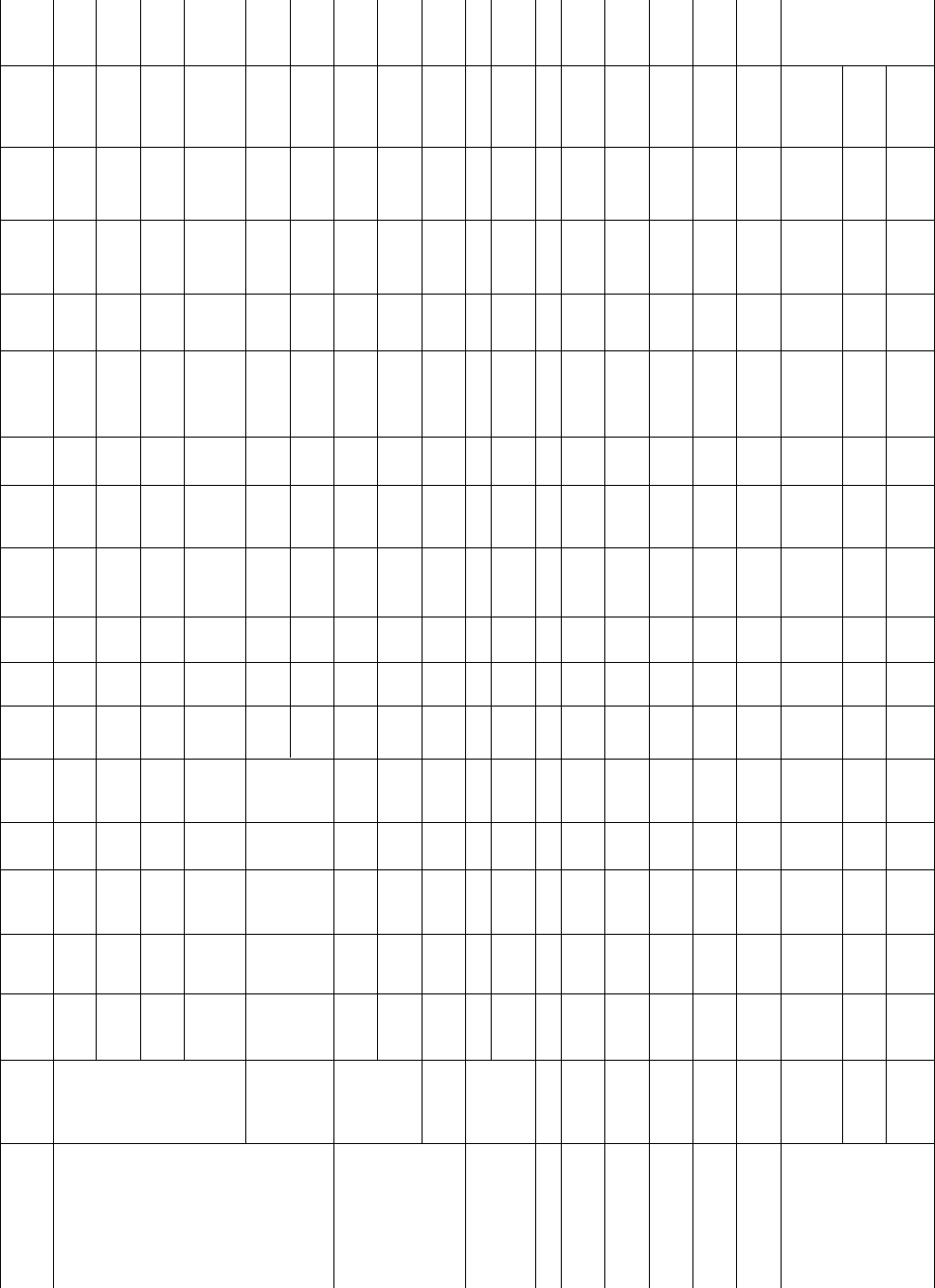
TABLE 39.3.

Continued.

Polymer

(kg=mol)

kg=mol

(



(



(J=g)

Growth

face

)



(cal=mol)

Regime

(



(cm=s)

=10

)

(erg

=cm

)

(erg=cm

)

(kcal

=mol)

Ref.

Polypropylene

iPP

350 

209 (110) 5.49 6.26 1,500 II

:40  10

1

11.5 62.3

[91]

186.1

(040) 6.56 5.24

III 138 3

:98  10

72 257

12 186.1 165 (110) 5.49 6.26 1,500

3:45  10

1

1.365 11.5 48.1

[92]

III 138.0 3

:03  10

3.659 11.5 59.0

300 600

3:4 185.0 8.3 (110) 5.49 6.26 1,500

1.250 11.5 51.3 5.07 [93]

(kJ/mol)

III 137

2.554 11.5 52.3 5.19

15 25.5

6:0 170.0 8.3 (110) 5.49 6.26 1,500

2.996 11.5 63.5 6.28 [93]

(kJ/mol)

II 133

1.607 11.5 68.2 6.74

III 122

3.196 11.5 67.7 6.69

sPP 76.2 165

6:1 168.7 177 (010) 7.25 5.60 1,500

III 110 9

:07 

5.69 11.28 124.5 14.6 [59]

(J=cm

) (200) 5.60 7.25

11.28 96.2 11.2

(020) 7.25 5.60 1,500 II

7.52 1.61 11.27 70.7 8.3

[94]

(200) 5.60 7.25

11.28 54.6 6.4

Polystyrene

iPS

90.5 242.0 91

(J=cm

)

12.8 5.5 1,560 II

1.20 7.64 34.8 7.1 [3]

9:1

(J=

)

(110) 12.8 5.5

1:31

 10

5.3 28.8

[95]

sPS 91.6 220 100 278.8

57:5 (040) 4.41 7.2 1,500 II

1.58 3.24 48.15 4.11 [63]

(J=cm

)

III 239

3.67 3.24 56.5 4.87

Poly(tetramethyl- PPSS

24:0 153.8

6.43 6.41 990

2:16 

1

1.14

34 4.0 [71]

- silphenylene)-

siloxane

or TMPS 286 372



24:0 152 20.8

6.41 1,230

1:03  10

1

3.5 36.3

[13–15]

Selenium

26.8 219.2

4.36 3.78 2,180

0:458 

2.53

190 9.0 [71]

Poly(tetrafluor

oethylene)

PTFE

184.6 331 47.4

1,500

0.154

[62]

Poly(arylene-

100 292

1,500 II

[64]

ether-ether-sulfide)

III 205

Poly(ester-amide)

21 170

2,800 II

1.63

[65]

III

3.15

Poly(vinylidene

fluoride)

PVDF 170

178 201

=cm

)

4.83

9.7 38

[69]

1, 2-Syndiotactic

polybutadiene

1,2-sPB

18 208

1,500 II

[70]

Ethylene-octene

139.3

[19]

copolymers L

 04

27.3 59.9

1.500 II 119.5

(random,

III 113.5

metallocene) H

 07

43.6 94

134.1

1,500 II

III 115.1

L  11

21.2 43.7

134.9

1,500 II

III 114.2