Masujima M. Applied Mathematical Methods in Theoretical Physics
Подождите немного. Документ загружается.


196 6 Singular Integral Equations of the Cauchy Type
hence we obtain the homogeneous solution to be
H (z) = G(z)exp
1
2
ln
b − z
a − z
= G(z)
b − z
a − z
. (6.1.21)
Suppose we choose
G(z) = 1(b − z),
so that
H (z) = 1
(b − z)(a − z). (6.1.22)
Therefore,
1H(z) =
(b − z)(a − z)
does not blow up at z = a or b. So, it is a good choice, since it does not make
f (x)H
+
(x)blowupanyfasterthanf (x)itself.HencewetakeEq.(6.1.22)forH(z).
Take that branch of H(z) f or which on the upper bank of the cut, we have
H
+
(x) = 1i
(b − x)(x − a),
where we have now the usual real square root. To do this, we set
z = a + r
1
e
iθ
1
and z = b + r
2
e
iθ
2
,
so that
(b − z)(z − a) =
√
r
1
r
2
exp(i
θ
1
+ θ
2
2
).
On x ∈ [a, b], we have
√
r
1
r
2
=
(b − x)(x − a) which requires on the upper bank,
exp(i
θ
1
+ θ
2
2
) = i.
We take on the upper bank θ
1
= 0andθ
2
= π.Thuswehave
H
+
(x) = 1i
(b − x)(x − a)andH
−
(x) =−1i
(b − x)(x − a ).
(6.1.23)
Step 2. Now look at the inhomogeneous problem:
+
(x) =−
−
(x) + f (x). (6.1.24)

6.2 Cauchy Integral Equation of the First Kind 197
Seek for the solution of the form
(
z
)
= H
(
z
)
K
(
z
)
. (6.1.25)
Then we have
H
+
(x)K
+
(x) =−H
−
(x)K
−
(x) + f (x) = H
+
(x)K
−
(x) + f (x),
where Eq. (6.1.19) has been used. Dividing both sides of the above equation by
H
+
(x), we have
K
+
(x) − K
−
(x) = f (x)H
+
(x) = i
(b − x)(x − a)f (x). (6.1.26)
By applying the discontinuity formula, we obtain
K(z) =
1
2πi
b
a
i
(b − x)(x − a)f (x)
x − z
dx + g(z), (6.1.27)
where g(z) is an arbitrary function with no cut on [a, b]. Thus the final solution is
given by
(z) = H(z)K(z)
=
1
(b − z)(a − z)
1
2π
b
a
(b − x)(x − a)f (x)
x − z
dx + g(z)
,
or equivalently
(
z
)
= H (z)
1
2πi
b
a
f (x)
H
+
(x)(x − z)
dx + g(z)
. (6.1.28)
6.2
Cauchy Integral Equation of the First Kind
Consider now the inhomogeneous Cauchy integral equation of the first kind:
1
πi
P
b
a
φ(y)
y − x
dy = f (x), a < x < b . (6.2.1)
Define
(
z
)
≡
1
2πi
b
a
φ(y)
y − z
dy for z not on [a, b]. (6.2.2)
198 6 Singular Integral Equations of the Cauchy Type
As z approaches the branch cut from above and below, we find
+
(x) =
1
2πi
P
b
a
φ(y)
y − x
dy +
1
2
φ(x), (6.2.3a)
−
(x) =
1
2πi
P
b
a
φ(y)
y − x
dy −
1
2
φ(x). (6.2.3b)
Adding (6.2.3a) and (6.2.3b) and subtracting (6.2.3b) from (6.2.3a) results in
+
(x) +
−
(x) =
1
πi
P
b
a
φ(y)
y − x
dy = f (x), (6.2.4)
+
(x) −
−
(x) = φ(x). (6.2.5)
Our strategy is the following. Solve Eq. (6.2.4) (which is the inhomogeneous Hilbert
problem) to find (z). Then use Eq. (6.2.5) to obtain φ(x). We remark that (z)
defined above is analytic in C − [a, b], so it can have no other singularities. Also
note that it behaves as Az as |z|→∞.
Solution.
+
(x) =−
−
(x) + f (x), a < x < b.
This is the inhomogeneous Hilbert problem that we solved in Section 6.2. We know
(z) = H(z)
1
2πi
b
a
f (x)
H
+
(x)(x − z)
dx + g(z)
. (6.2.6)
However, we can say something about the form of g(z) in this case by examining
the behavior of (z)as|z|→∞. By our original definition of (z), we have
(z) ∼ Az as
|
z
|
→∞, (6.2.7a)
with
A =−
1
2πi
b
a
φ(y)dy. (6.2.8)
If we examine the above solution, upon noting that
H (z) ∼ 1z as
|
z
|
→∞,
wefindthatithastheasymptoticform
(z) ∼ O(1z
2
) + g(z)z as
|
z
|
→∞. (6.2.7b)
6.2 Cauchy Integral Equation of the First Kind 199
Now, since (z) is analytic everywhere away from the branch cut [a, b], we conclude
that g(z)H(z) must also be analytic away from the cut [a, b]. Other singularities
of g(z)on[a, b] can also be excluded. Hence g(z) must be entire. Comparing
the asymptotic forms (6.2.7a) and (6.2.7b), we conclude g(z) → A as |z|→∞.
Therefore, by Liouville’s theorem, we must have g(z) = A identically. Therefore,
we have
(z) = H(z)
1
2πi
b
a
f (x)
H
+
(x)(x − z)
dx + A
. (6.2.9)
Thus we have
+
(x) = H
+
(x)
1
2πi
P
b
a
f (y)
H
+
(y)(y − x)
dy +
1
2
f (x)
H
+
(x)
+ A
, (6.2.10a)
−
(x) =−H
+
(x)
1
2πi
P
b
a
f (y)
H
+
(y)(y − x)
dy −
1
2
f (x)
H
+
(x)
+ A
. (6.2.10b)
Hence φ(x)isgivenby
φ
(
x
)
=
+
(x) −
−
(x) = H
+
(x)
1
πi
P
b
a
f (y)
H
+
(y)(y − x)
dy + 2AH
+
(x).
(6.2.11)
Note that
H
+
(x) = 1
(b − x)(a − x) = 1i
(b − x)(x − a). (6.2.12)
The second term on the right-hand side of φ(x) turns out to be the solution of the
homogeneous problem. So A is arbitrary. In order to understand this point more
completely, it makes sense to examine the homogeneous problem separately.
Consider the homogeneous Cauchy integral equation of the first kind:
1
πi
P
b
a
φ(y)
y − x
dy = 0. (6.2.13)
Define
(
z
)
≡
1
2πi
b
a
φ(y)
y − z
dy.
(z) is analytic everywhere away from [a, b], and it has the asymptotic behavior
(
z
)
∼ Az as
|
z
|
→∞,
with
A =−
1
2πi
b
a
φ(y)dy. (6.2.14)
200 6 Singular Integral Equations of the Cauchy Type
We have
+
(x) =
1
2πi
P
b
a
φ(y)
y − x
dy +
1
2
φ
(
x
)
,
−
(
x
)
=
1
2πi
P
b
a
φ(y)
y − x
dy −
1
2
φ
(
x
)
.
From these, we obtain
+
(
x
)
+
−
(
x
)
= 0, (6.2.15 a)
+
(x) −
−
(x) = φ(x). (6.2.15b)
Solve
+
(x) =−
−
(x),
which is the homogeneous Hilbert problem whose solution (z)wealreadyknow
from Section 6.2. Namely, we have
(
z
)
= G(z)
b − z
a − z
, (6.2.16)
with G(z)havingnobranchcutson[a, b]. But in this case, we can determine the
form of G(z).
(i) We know that (z)isanalyticawayfrom[a, b], so G(z)canonlyhave
singularities on [a, b], but has no branch cuts there.
(ii) We know
(
z
)
∼ Az as
|
z
|
→∞,
so G(z) must also behave as
G(z) ∼ Az as
|
z
|
→∞,
taking that branch of
(b − z)(a − z)whichgoesto+1as|z|→∞.
(iii) (z) can only be singular at the end points and then not as bad as a pole,
since it is of the form
1
2πi
b
a
φ(y)
y − z
dy.
So, G(z) may only be singular at the end points a or b.

6.3 Cauchy Integral Equation of the Second Kind 201
The last condition (iii), together with the asymptotic form of G(z)as|z|→∞,
suggests functions of the form
(a − z)
n
(b − z)
n+1
or
(b − z)
n
(a − z)
n+1
.
The only choice for which the resulting (z) does not blow up as bad as a pole at
the two end points is
G(z) = A(b − z)withA = arbitrary constant. (6.2.17)
Therefore, the form of (z) is d etermined to be
(
z
)
= A
(b − z)(a − z). (6.2.18)
Then the homogeneous solution is given by
φ
(
x
)
=
+
(x) −
−
(x) = 2
+
(x) = 2A
(b − x)(a − x ) = 2AH
+
(x),
(6.2.19)
where H
+
(x) is given by Eq. (6.2.12). To verify that any A works, recall Eq. (6.2.14),
A =−
1
2πi
b
a
φ(y)dy.
Substituting φ(y) just obtained, Eq. (6.2.19), into the above expression for A,we
have
A =−
2A
2πi
b
a
dy
(b − y)(a − y)
=
A
π
b
a
dy
(b − y)(y − a)
=
A
π
+1
−1
dξ
1 − ξ
2
= A,
which is true for any A.
6.3
Cauchy Integral Equation of the Second Kind
We now consider the inhomogeneous Cauchy integral equation of the second kind,
φ(x) = f (x) +
λ
π
P
1
0
φ(y)
y − x
dy,0< x < 1. (6.3.1)
Define (z)
(z) ≡
1
2πi
1
0
φ(y)
y − z
dy. (6.3.2)
202 6 Singular Integral Equations of the Cauchy Type
The boundary values of (z)asz approaches the cut [0, 1] from above and below
are given, respectively, by
+
(x) =
1
2πi
P
1
0
φ(y)
y − x
dy +
1
2
φ(x), 0 < x < 1,
−
(x) =
1
2πi
P
1
0
φ(y)
y − x
dy −
1
2
φ(x), 0 < x < 1,
so that
+
(x) −
−
(x) = φ(x), 0 < x < 1, (6.3.3)
+
(x) +
−
(x) =
1
πi
P
1
0
φ(y)
y − x
dy,0< x < 1. (6.3.4)
Equation (6.3.1) now reads
+
(x) −
−
(x) = f (x) + iλ(
+
(x) +
−
(x)),
or
+
(x) −
1 + iλ
1 − iλ
−
(x) =
1
1 − iλ
f (x). (6.3.5)
Werecognizethisastheinhomogeneous Hilbert problem.
Consider the case λ>0andsetλ equal to
λ = tan πγ,0<γ ≤
1
2
. (6.3.6)
Then we have
1 + iλ
1 − iλ
= e
2πiγ
.
First, we solve a homogeneous problem:
H
+
(x) = H
−
(x)e
2πiγ
,0< x < 1. (6.3.7)
In terms of h(z)definedby
H (z) = e
h(z)
,
we have
h
+
(x) − h
−
(x) = 2π iγ.
6.3 Cauchy Integral Equation of the Second Kind 203
Hence we obtain
h(z) =
1
2πi
1
0
2πiγ
y − z
dz = γ ln
1 − z
−z
,
and
H (z) =
1 − z
−z
γ
,0<γ ≤ 1 2. (6.3.8)
Since we can add any function with no cut on [0, 1] to h(z), we can multiply any
function with no cut on [0, 1] onto H(z). By multiplying the above equation by
e
iπγ
(1 − z), we choose
H (z) = 1[(1 − z)
1−γ
z
γ
], 0 <γ ≤ 12. (6.3.9)
Returning to the inhomogeneous Hilbert problem, Eq. (6.3.5), we write
(z) = H(z)G(z). (6.3.10)
Then Eq. (6.3.5) reads
H
+
(x)G
+
(x) − H
+
(x)G
−
(x) =
1
1 − iλ
f (x).
Dividing through the above equation by H
+
(x), we have
G
+
(x) − G
−
(x) =
1
1 − iλ
f (x)H
+
(x) =
1
1 − iλ
f (x)(1 − x)
1−γ
x
γ
. (6.3.11)
Since, for our choice of H(z), Eq. (6.3.9), we have
1H
+
(0) = 1H
+
(1) = 0,
we did not bring in extra singular behavior at x = 0 and 1; rather we made
f (x)H
+
(x) better behaved than f (x)atx = 0 and 1. By the discontinuity formula,
we have
G(z) =
1
2πi
1
1 − iλ
1
0
[f (y)(1 − y)
1−γ
y
γ
(y − z)]dy + g(z). (6.3.12)
The integral on the right-hand side of Eq. (6.3.12) takes care of the discontinuity of
G(z) across the cut on [0, 1] so that g(z) does not have any cut on [0, 1]. We know
furthermore that

204 6 Singular Integral Equations of the Cauchy Type
(1) G(z) is analytic in the cut z plane.
(2) As z → 0, G(z)isboundedby
G(z)
<
1
z
α
· z
γ
,
and similarly for z → 1.
(3) As |z|→∞, G(z) is bounded by constant. Thus we know from Eq. (6.3.12)
that g(z) is analytic everywhere and
g(z) ∼ constant as
|
z
|
→∞.
By Liouville’s theorem, we obtain
g(z) = constant = k. (6.3.13)
Henceweobtain
(z) =
1
(1 − z)
1−γ
z
γ
1
2πi
1
1 − iλ
1
0
(1 − y )
1−γ
y
γ
y − z
f (y)dy +
k
(1 − z)
1−γ
z
γ
.
(6.3.14)
Then by choosing the branch of H(z) as indicated in Figure 6.1, we have from the
Plemelj formula
+
(x) =
1
2πi
1
1 − iλ
1
(1 − x)
1−γ
x
γ
P
1
0
(1 − y )
1−γ
y
γ
y − x
f (y)dy +
1
2
1
1 − iλ
f (x)
+
k
(1 − x)
1−γ
x
γ
, (6.3.15a)
−
(x) =
1
2πi
1
1 − iλ
e
−2πiγ
(1 − x)
1−γ
x
γ
P
1
0
(1 − y )
1−γ
y
γ
y − x
f (y)dy −
1
2
e
−2πiγ
1 − iλ
f (x)
+
ke
−2πiγ
(1 − x)
1−γ
x
γ
. (6.3.15b)
By Eq. (6.3.3),
φ(x) =
+
(x) −
−
(x)
=
1
2πi
1 − e
−2πiγ
1 − iλ
1
(1 − x)
1−γ
x
γ
P
1
0
(1 − y )
1−γ
y
γ
y − x
f (y)dy
+
1
2
1 + e
−2πiγ
1 − iλ
f (x) +
c
(1 − x)
1−γ
x
γ
. (6.3.16)
6.4 Carleman Integral Equation 205
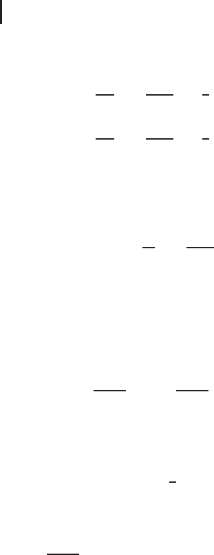
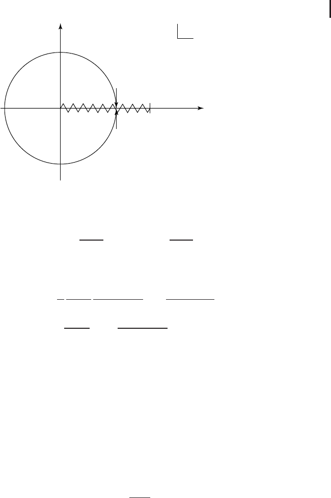
Z
o
1
Z
=
x
Z
=
e
2p
i
x
Fig. 6.1 The branch of H(z) chosen for Eqs. (6.3.15a) and (6.3.15b).
Sincewehave
1 − e
−2πiγ
=
2iλ
1 + iλ
,1+ e
−2πiγ
=
2
1 + iλ
,
we finally obtain
φ(x) =
1
π
λ
1 + λ
2
1
(1 − x)
1−γ
x
γ
P
1
0
(1 − y )
1−γ
y
γ
y − x
f (y)dy
+
1
1 + λ
2
f (x) +
c
(1 − x)
1−γ
x
γ
, (6.3.17)
where c is an arbitrary constant. We note that solution (6.3.17) involves one
arbitrary constant and the spectrum of the eigenvalue λ of Eq. (6.3.1) with f (x) ≡ 0
is continuous. It is noted that the homogeneous solution of Eq. (6.3.1) with f (x) ≡ 0
comes from the entire function g(z).
6.4
Carleman Integral Equation
Consider the inhomogeneous Carleman integral equation
a(x )φ(x) = f (x) + λP
+1
−1
φ(y)
y − x
dy, − 1 < x < 1, (6.4.1)
which has a Cauchy kernel and is a generalization of the Cauchy integral equation
of the second kind. Assume that λ is real and that f (x)anda(x) are prescribed real
functions. Without loss of generality, we can take λ>0(otherwise,wejustchange
the sign of a(x)andf (x)).