McConnell Campbell R., Brue Stanley L., Barbiero Thomas P. Microeconomics. Ninth Edition

Подождите немного. Документ загружается.

350 Part Two • Microeconomics of Product Markets

internet application question

1. Visit Canada’s Competition Tribunal’s Web

site at <www.ct-tc.gc.ca/english/current.html>.

Review the current ﬁlings. What companies

does the latest ﬁling include? Scroll down to

“Decision Rendered.” Review the case of the

Bank of Montreal. On what basis did the Com-

missioner of Competition make its decision?

from marginal-cost pricing, which pricing

policy would you favour? Why? What prob-

lems might such a subsidy entail?

10.

KEY QUESTION How does social

regulation differ from industrial regulation?

What types of beneﬁts and costs are associ-

ated with social regulation?

11. Use economic analysis to explain why the

optimal amount of product safety may be

less than the amount that would totally elim-

inate risks of accidents and deaths. Use auto-

mobiles as an example.

12. (The Last Word) Under what law and on

what basis did the U.S. federal govern-

ment ﬁnd Microsoft guilty of violating U.S.

antitrust laws? What was the government’s

proposed remedy? In mid-2000 Microsoft

appealed the District Court decision to a

higher court. Update the Microsoft story,

using an Internet search engine. What is the

current status of that appeal? Is it still pend-

ing? Did Microsoft win its appeal? Or was the

District Court’s decision upheld?

IN THIS CHAPTER

OU WILL LEARN:

How resource prices

are determined.

•

What determines the

demand for a resource.

•

What determines the

elasticity of resource demand.

•

How to arrive at the optimal

combination of resources to

use in the production process.

The Demand

for Resources

e now turn from the pricing and

production of goods and services

to the pricing and employment of

resources. Although ﬁrms come in various

sizes and operate under highly different mar-

ket conditions, they each have a demand

for productive resources. They obtain those

resources from households—the direct or

indirect owners of land, labour, capital, and

entrepreneurial resources. So, referring to

the circular ﬂow model (Figure 2-6), we shift

our attention from the bottom loop of the

diagram (where businesses supply products

that households demand) to the top loop

(where businesses demand resources that

households supply).

FOURTEEN

This chapter looks at the demand for economic resources. Although the discussion is

couched in terms of labour, the principles we develop also apply to land, capital,

and entrepreneurial ability. In Chapter 15 we will combine resource (labour)

demand with labour supply to analyze wage rates. Then in Chapter 16 we will use

resource demand and resource supply to examine the prices of, and returns to, other

productive resources.

There are several good reasons to study resource pricing:

● Money-income determination Resource prices are a major factor in deter-

mining the income of households. The expenditures that ﬁrms make in acquir-

ing economic resources ﬂow as wage, rent, interest, and proﬁt incomes to the

households that supply those resources.

● Resource allocation Just as product prices allocate ﬁnished goods and serv-

ices to consumers, resource prices allocate resources among industries and

ﬁrms. In a dynamic economy, where technology and tastes often change,

the efﬁcient allocation of resources over time calls for the continuing shift of

resources from one use to another. Resource pricing is a major factor in pro-

ducing those shifts.

● Cost minimization To the ﬁrm, resource prices are costs, and to realize max-

imum proﬁt, the ﬁrm must produce the proﬁt-maximizing output with the

most efﬁcient (least costly) combination of resources. Resource prices play the

main role in determining the quantities of land, labour, capital and entrepre-

neurial ability that will be combined in producing each good or service.

● Ethical questions and policy issues

Many ethical questions and public policy

issues surround the resource market. What degree of income inequality is accept-

able? Should the government levy a special tax on the excess pay of corporate ex-

ecutives? Should the federal government establish a legal minimum wage? Does

it make sense for the government to provide subsidies to farmers? The facts, ethics,

and debates relating to income distribution are all based on resource pricing.

To make things simple, we will ﬁrst assume that a ﬁrm hires a certain resource in a

purely competitive resource market and sells its output in a purely competitive

product market. The simplicity of this situation is twofold: In a competitive prod-

uct market the ﬁrm is a price-taker and can dispose of as little or as much output as

it chooses at the market price. The ﬁrm is selling such a negligible fraction of total

output that it exerts no inﬂuence on product price. Similarly, in the competitive

resource market, the ﬁrm is a wage-taker. It hires such a negligible fraction of the

total supply of the resource that it cannot inﬂuence the resource price.

Resource Demand as a Derived Demand

The demand for resources is a derived demand: it is derived from the products that

those resources help produce. Resources usually do not directly satisfy customer

chapter fourteen • the demand for resources 353

Signiﬁcance of Resource Pricing

Marginal Productivity Theory

of Resource Demand

derived

demand

The demand for

a resource that

depends on the

products it can be

used to produce.

<www.rci.rutgers.edu/

~gag/NOTES/

micnotes11.html>

Marginal productivity

theory of distribution

Choosing

a Little More

or Less

wants but do so indirectly through their use in producing goods and services. No one

wants to consume a hectare of land, a John Deere tractor, or the labour services of a

farmer, but households do want to consume the food and ﬁbre products that these

resources help produce. Similarly, the demand for airplanes generates a demand for

assemblers, and the demands for such services as income-tax preparation, haircuts,

and child care create derived demands for accountants, barbers, and child-care work-

ers. Global Perspective 14.1 demonstrates that the global demand for labour is derived.

Marginal Revenue Product (MRP)

The derived nature of resource demand means that the strength of the demand for

any resource will depend on

● the productivity of the resource in helping to create a good

● the market value or price of the good it helps to produce

A resource that is highly productive in turning out a highly valued commodity will

be in great demand, while a relatively unproductive resource that is capable of pro-

ducing only a slightly valued commodity will be in little demand. There will be no

demand at all for a resource that is phenomenally efﬁcient in producing something

that no one wants to buy.

PRODUCTIVITY

Table 14-1 shows the roles of productivity and product price in determining

resource of demand. Here, we assume that a ﬁrm adds one variable resource,

labour, to its ﬁxed plant. Columns 1 and 2 give the number of units of the resource

354 Part Three • Microeconomics of Resource Markets

Labour demand and

allocation: developing

countries, industrially

advanced countries,

and Canada

The idea of derived demand

implies that the composition

of a country’s product-market

demand will determine the allo-

cation of its labour force among

agricultural products, industrial

goods, and services. Because

lower-income nations must spend most of their incomes on food and ﬁbre,

the bulk of their labour is allocated to agriculture. The industrially advanced

economies with higher incomes allocate most of their labour to industrial

products and services.

14.1

Percentage of Labour Force

250 50 75 100

Developing

countries

Industrially

advanced

countries

Canada

Agriculture

Industry

Services

Agriculture

Industry

Services

Agriculture

Industry

Services

Source: International Labour Organization data, <www.ilo.org>.

applied to production and the resulting total product (output). Column 3 provides

the marginal product (MP), or additional output, resulting from each additional

resource unit. Columns 1 through 3 remind us that the law of diminishing returns

applies here, causing the marginal product of labour to fall beyond some point. For

simplicity, we assume that those diminishing marginal returns—those declines in

marginal product—begin after the ﬁrst worker hired.

PRODUCT PRICE

The derived demand for a resource depends also on the price of the commodity it

produces. Column 4 in Table 14-1 adds this price information. Product price is con-

stant, in this case at $2, because we are assuming a competitive product market. The

ﬁrm is a price-taker and will sell units of output only at this market price.

Multiplying column 2 by column 4 gives us the total-revenue data of column 5.

These are the amounts of revenue the ﬁrm realizes from the various levels of

resource usage. From these total-revenue data we can compute marginal revenue

product (MRP), the change in total revenue resulting from the use of each addi-

tional unit of a resource (labour, in this case). In equation form,

Marginal revenue product =

The MRPs are listed in column 6 in Table 14-1.

Rule for Employing Resources: MRP = MRC

The MRP schedule, shown as columns 1 and 6, is the ﬁrm’s demand schedule for labour. To

explain why, we must ﬁrst discuss the rule that guides a proﬁt-seeking ﬁrm in hir-

ing any resource: To maximize proﬁt, a ﬁrm should hire additional units of a speciﬁc

resource as long as each successive unit adds more to the ﬁrm’s total revenue than it adds to

total cost.

Economists use special terms to designate what each additional unit of labour or

other variable resource adds to total cost and what it adds to total revenue. We have

seen that MRP measures how much each successive unit of a resource adds to total

change in total revenue

ᎏᎏᎏᎏᎏ

one unit change in resource quantity

TABLE 14-1 THE DEMAND FOR LABOUR: PURE COMPETITION

IN THE SALE OF THE PRODUCT

(1) (2) (3) (4) (5) (6)

Units of Total Marginal Product Total Marginal

resource product product, MP price revenue, or revenue

(output) (2) × (4) product, MRP

$2 $ 0

$14

214

213

226

318

236

422

244

525

250

627

254

728 256

chapter fourteen • the demand for resources 355

marginal

product

(MP)

The extra

output produced

with one additional

unit of a resource.

marginal

revenue

product

(MRP)

The

change in total

revenue from

employing one

additional unit of

a resource.

revenue. The amount that each additional unit of a resource adds to the ﬁrm’s total

(resource) cost is called its marginal resource cost (MRC).

In equation form,

Marginal resource cost =

So we can restate our rule for hiring resources as follows: It will be proﬁtable for

a ﬁrm to hire additional units of a resource up to the point at which that resource’s

MRP is equal to its MRC. If the number of workers a ﬁrm is currently hiring is such

that the MRP of the last worker exceeds his or her MRC, the ﬁrm can proﬁt by hir-

ing more workers. But if the number being hired is such that the MRC of the last

worker exceeds his or her MRP, the ﬁrm is hiring workers who are not paying their

way, and it can increase its proﬁt by discharging some workers. You may have rec-

ognized that this MRP = MRC rule is similar to the MR = MC proﬁt-maximizing

rule employed throughout our discussion of price and output determination. The

rationale of the two rules is the same, but the point of reference is now inputs of a

resource, not outputs of a product.

MRP as Resource Demand Schedule

In a purely competitive labour market, supply and demand establish the wage rate.

Because each ﬁrm hires such a small fraction of market supply, it cannot inﬂuence

the market wage rate; it is a wage-taker, not a wage-maker. This means that for each

additional unit of labour hired, total resource cost increases by exactly the amount

of the constant market wage rate. The MRC of labour exactly equals the market

wage rate. Thus, resource “price” (the market wage rage) and resource “cost” (mar-

ginal resource cost) are equal for a ﬁrm that hires a resource in a competitive labour

market. Then the MRP = MRC rule tells us that, in pure competition, the ﬁrm will hire

workers up to the point at which the market wage rate (its MRC) is equal to its MRP.

In terms of the data in columns 1 and 6 in Table 14-1, if the market wage rate is,

say, $13.95, the ﬁrm will hire only one worker, because the ﬁrst worker adds $14 to

total revenue and slightly less—$13.95—to total cost. In other words, because MRP

exceeds MRC for the ﬁst worker, it is proﬁtable to hire that worker. For each suc-

cessive worker, however, MRC (= $13.95) exceeds MRP (= $12 or less), indicating

that it will not be proﬁtable to hire any of those workers. If the wage rate is $11.95,

by the same reasoning we discover that it will pay the ﬁrm to hire both the ﬁrst and

second workers. Similarly, if the wage rate is $9.95, three will be hired. If $7.95, four.

If $5.95, ﬁve. And so forth. Hence, the MRP schedule constitutes the ﬁrm’s demand for

labour, because each point on this schedule (or curve) indicates the number of workers the

ﬁrm would hire at each possible wage rate. In Figure 14-1, we show the D = MRP curve

based on the data in Table 14-1.

The logic here will be familiar to you: In Chapter 9 we applied the price-equals-

marginal-cost (P = MC) rule for proﬁt-maximizing output to discover that the por-

tion of the purely competitive ﬁrm’s short-run marginal-cost curve lying above

the AVC curve is the short-run product supply curve. Here, we are applying the

MRP = MRC (= resource price) rule for proﬁt-maximizing input to discover that

the purely competitive ﬁrm’s MRP curve is its resource demand curve.

Resource Demand under Imperfect Product Market Competition

Our analysis of labour demand becomes more complex when the ﬁrm is selling its

product in an imperfectly competitive market, one in which the ﬁrm is a price-

change in total (resource) cost

ᎏᎏᎏᎏᎏ

one unit change in resource quantity

356 Part Three • Microeconomics of Resource Markets

marginal

resource

cost (MRC)

The amount that

each additional unit

of resource adds

to the ﬁrm’s total

(resource) cost.

mrp = mrc

rule

To maxi-

mize economic

proﬁt (or minimize

losses) a ﬁrm

should use the

quantity of a

resource at which

its marginal rev-

enue product is

equal to its mar-

ginal resource cost.

<cepa.newschool.edu/

het/essays/margrev/

distrib.htm#marginal>

Marginal productivity

theory of distribution

maker. Pure monopoly, oligopoly, and monopolistic competition in the product

market all mean that the ﬁrm’s product demand curve is downsloping; the ﬁrm

must set a lower price to increase its sales.

The productivity data in Table 14-1 are retained in columns 1 to 3 in Table 14-2.

But here we show in column 4 that product price must be lowered to sell the mar-

ginal product of each successive worker. The MRP of the purely competitive seller

of Table 14-1 falls for one reason: marginal product diminishes. The MRP of the

imperfectly competitive seller of Table 14-2 falls for two reasons: marginal product

diminishes and product price falls as output increases.

We emphasize that the lower price accompanying each increase in output (total

product) applies not only to the marginal product of each successive worker but also

chapter fourteen • the demand for resources 357

FIGURE 14-1 THE PURELY COMPETITIVE SELLER’S DEMAND

FOR A RESOURCE

$14

01234

= MRP

Resource price (wage rate)

Quantity of resource demanded

The MRP curve is the

resource demand curve;

each of its points relates a

particular resource price

(= MRP when proﬁt is maxi-

mized) with a corresponding

quantity of the resource

demanded. Under pure

competition, product price

is constant; therefore, the

downward slope of the D =

MRP curve is due solely to

the decline in the resource’s

marginal product (law of

diminishing marginal

returns).

TABLE 14-2 THE DEMAND FOR LABOUR: IMPERFECT

COMPETITION IN THE SALE OF THE PRODUCT

(1) (2) (3) (4) (5) (6)

Units of Total Marginal Product Total Marginal

resource product product, MP price revenue, or revenue

(output) (2) × (4) product, MRP

$2.80 $ 0

$18.20

2.60 18.20

13.00

213

2.40 31.20

8.40

318

2.20 39.60

4.40

422

2.00 44.00

2.25

525

1.85 46.25

1.00

627

1.75 47.25

–1.05

7 28 1.65 46.20

to all prior output units that otherwise could have been sold at a higher price. Note that

the second worker’s marginal product is six units. These six units can be sold for

$2.40 each, or, as a group, for $14.40. But this is not the MRP of the second worker.

To sell these six units, the ﬁrm must take a 20-cent price cut on the seven units

produced by the ﬁrst worker—units that otherwise could have been sold for $2.60

each. Thus, the MRP of the second worker is only $13.00 [= $14.40 – (7 × 20 cents)],

as shown.

Similarly, the third worker adds ﬁve units to total product, and these units are

worth $2.20 each, or $11.00 total. But to sell these ﬁve units the ﬁrm must take a 20-

cent price cut on the 13 units produced by the ﬁrst two workers. So the third

worker’s MRP is only $8.40 [= $11.00 – (13 × 20 cents)]. The other ﬁgures in column

6 are derived in the same way.

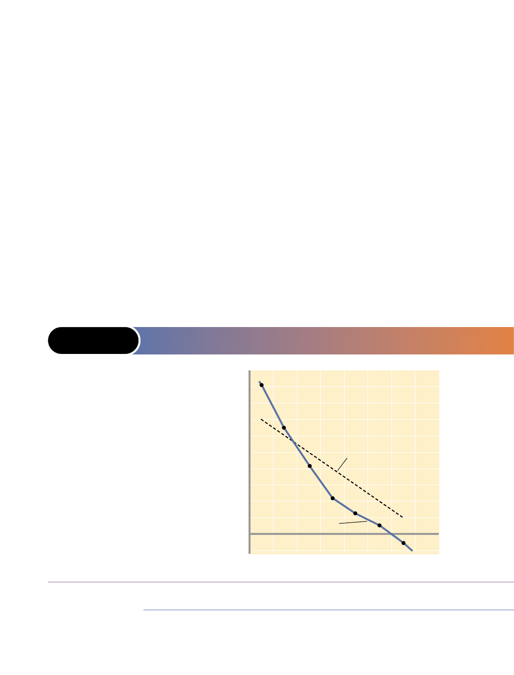
The result is that the MRP curve—the resource demand curve—of the imperfectly

competitive producer is less elastic than that of the purely competitive producer. At

a wage rate or MRC of $11.95, both the purely competitive and the imperfectly com-

petitive seller will hire two workers. But at $9.95 the competitive ﬁrm will hire three,

and the imperfectly competitive ﬁrm only two. At $7.95 the purely competitive ﬁrm

will employ four employees, and the imperfect competitor only three. You can see

this difference in resource demand elasticity when we graph the MRP data in Table

14-2 and compare the graph with Figure 14-1, as we do in Figure 14-2.

358 Part Three • Microeconomics of Resource Markets

Note that we plot the points in Figures 14-1 and 14-2 halfway between succeeding numbers of

resource units, because MRP is associated with the addition of one more unit. Thus, in Figure

14-2, for example, we plot the MRP of the second unit ($13.00) not at one or two, but rather at 1.5.

This smoothing enables us to sketch a continuously downsloping curve rather than one that

moves downward in discrete steps as each new unit of labour is hired.

FIGURE 14-2 THE IMPERFECTLY COMPETITIVE SELLER’S DEMAND

CURVE FOR A RESOURCE

$18

–2

1234

Quantity of resource demanded

Resource price (wage rate)

= MRP

(pure competition)

= MRP

(imperfect

competition)

An imperfectly

competitive seller’s

resource demand

curve D (solid) slopes

downward because

both marginal prod-

uct and product price

fall as resource

employment and out-

put rise. This down-

ward slope is greater

than that for a purely

competitive seller

(dashed resource

demand curve)

because the pure

competitor can sell

the added output at

a constant price.

It is not surprising that the imperfectly competitive producer is less responsive

to resource price cuts than the purely competitive producer. The imperfect com-

petitor’s relative reluctance to employ more resources, and produce more output,

when resource prices fall reﬂects the imperfect competitor’s tendency to restrict out-

put in the product market. Other things equal, the imperfectly competitive seller

produces less of a product than a purely competitive seller. In producing that

smaller output, it demands fewer resources.

But there is one important qualiﬁcation. We noted in Chapter 11 that the market

structure of oligopoly might lead to technological progress and greater production,

more employment, and lower prices in the very long run than would a purely com-

petitive market. The resource demand curve in these cases would lie farther to the

right than it would if output were restricted as a result of monopoly power. (Key

Question 2)

Market Demand for a Resource

We have now explained the individual ﬁrm’s demand curve for a resource. Recall

that the total, or market, demand curve for a product is found by summing horizon-

tally the demand curves of all individual buyers in the market. The market demand

curve for a particular resource is derived in essentially the same way—by summing

the individual demand or MRP curves for all ﬁrms hiring that resource.

What will alter the demand for a resource—that is, shift the resource demand

curve? The fact that resource demand is derived from product demand and depends

on resource productivity suggests two things can shift resource demands. Also, our

analysis of how changes in the prices of other products can shift a product’s demand

curve (Chapter 3) suggests another factor: changes in the prices of other resources.

Changes in Product Demand

Other things equal, an increase in the demand for a product that uses a particular resource

will increase the demand for the resource whereas a decrease in product demand will decrease

the resource demand.

chapter fourteen • the demand for resources 359

Determinants of Resource Demand

● To maximize proﬁt a ﬁrm will use a resource in

an amount at which the resource’s marginal

revenue product equals its marginal resource

cost (MRP = MRC).

● Application of the MRP = MRC rule to a ﬁrm’s

MRP curve demonstrates that the MRP curve is

the ﬁrm’s resource demand curve. In a purely

competitive resource market, resource price

(the wage rate) equals MRC.

● The resource demand curve of a purely com-

petitive seller is downsloping solely because

the marginal product of the resource dimin-

ishes; the resource demand curve of an imper-

fectly competitive seller is downsloping because

marginal product diminishes and product price

falls as output is increased.

<www.theshortrun.com/

classroom/glossary/

micro/resource.html>

Resource demand

Let’s see how this works. The ﬁrst thing to recall is that a change in the demand

for a product will change its price. In Table 14-1, let’s assume that an increase in

product demand boosts the product price from $2 to $3. You should calculate the

new resource demand schedule (columns 1 and 6) that would result, and plot it in

Figure 14-1 to verify that the new resource demand curve lies to the right of the old

demand curve. Similarly, a decline in the product demand (and price) will shift the

resource demand curve to the left. This effect—resource demand changing along

with product demand—demonstrates that resource demand is derived from prod-

uct demand.

Changes in Productivity

Other things equal, an increase in the productivity of a resource will increase the demand

for the resource and a decrease in productivity will reduce the resource demand. If we

doubled the MP data of column 3 in Table 14-1, the MRP data of column 6 would

also double, indicating an increase (rightward shift) in the resource demand curve.

The productivity of any resource may be altered in several ways:

● Quantities of other resources The marginal productivity of any resource

will vary with the quantities of the other resources used with it. The greater the

amount of capital land resources used with, say, labour, the greater will be

labour’s marginal productivity and, thus, labour demand.

● Technological progress Technological improvements that increase the qual-

ity of other resources, such as capital, have the same effect. The better the qual-

ity of capital, the greater the productivity of labour used with it. Dockworkers

employed with a speciﬁc amount of real capital in the form of unloading

cranes are more productive than dockworkers with the same amount of real

capital embodied in older conveyer-belt systems.

● Quality of the variable resource Improvements in the quality of the variable

resource, such as labour, will increase its marginal productivity and therefore

its demand. In effect, there will be a new demand curve for a different, more

skilled, kind of labour.

All these considerations help explain why the average level of (real) wages is higher

in industrially advanced nations (for example, Canada, Germany, Japan, and

France) than in developing nations (for example, India, Ethiopia, Angola, and Cam-

bodia). Workers in industrially advanced nations are generally healthier, better edu-

cated, and better trained than are workers in developing countries. Also, in most

industries, workers in industrially advanced nations work with a larger and more

efﬁcient stock of capital goods and more abundant natural resources. This creates a

strong demand for labour. On the supply side of the market, labour is relatively

scarce compared with that in most developing nations. A strong demand and a rel-

atively scarce supply of labour result in high wage rates in the industrially advanced

nations.

Changes in the Prices of Other Resources

Just as changes in the prices of other products will change the demand for a speciﬁc

product, changes in the prices of other resources will change the demand for a spe-

ciﬁc resource. Also recall that the effect of a change in the price or product X on the

demand for product Y depends on whether X and Y are substitute goods or

360 Part Three • Microeconomics of Resource Markets