Molina-Par?s C., Lythe G. (editors) Mathematical Models and Immune Cell Biology
Подождите немного. Документ загружается.

9 Competing T Cell Clonotypes 203
and so
P
C1
kD1
d
k
converges by the ratio test. Hence, the series (9.38) converges by
comparison and so
n
is finite for all n 2 S nf.0;0;:::;0/g for all values of the
parameters.
Numerical Results
We have carried out numerical solutions of the competition model, without any type
of mean field approximation, using the Gillespie algorithm [14]. A number of T cell
clonotypes, N
c
, a number of APPs, jQj, and a set of connections between them, are
input at the start of a numerical run. In the run used to produce the data in Figs. 9.4
and 9.5, the initial number of T cell clonotypes is 1,000 and there are 100 cells of
each clonotype at t D 0. Connections between T cell clonotypes and APPs, meaning
that the clonotype receives a signal from the APP, are assigned independently with
probability p at the beginning of the run and not changed thereafter. The death rate
is constant; the birth rate of each clonotype is calculated using (9.6) at each time
during the numerical run. Each clonotype’s value of is a function of time that is the
average, over the APPs from which it receives a stimulus, of the number of other
surviving clonotypes also stimulated by an APP. A clonotype that only receives
signals from APPs that do not signal to any other clonotype will have D 0;a
clonotype that receives signals from two APPs, one of which signals to one other
clonotype and one of which signals to two other clonotypes, will have D 1:5.
0
400
800 N (t)
0
50
100
0
2
4
0 200 400 600 800
ν
t
ν
n
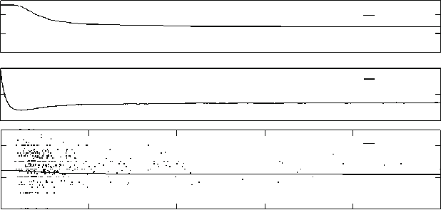
Fig. 9.4 Numerical results, showing the time evolution of the number of clonotypes with at least
one living cell, the mean number of cells per clonotype, and the mean value of . The T cell
clonotype–APP connections are randomly assigned at the beginning of the numerical run. The
parameters for the run are N
c
D 1;000, jQjD2;000, D 0:1, D 1 and p D 0:0025
204 C. Molina-Par´ıs et al.
400
800
0 1 2 3 4 5 6 7
APPs
T cell clonotypes signalled
01234567
T cell clonotypes signalled
start
0
400
800
APPs
end
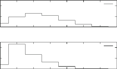
Fig. 9.5 Competition, and extinction of some clonotypes, leads to more uniform coverage of the
set of APPs by the repertoire of T cell clonotypes. The upper panel shows a histogram of the
number of clonotypes that recognise an APP at the beginning of the numerical run. The lower
panel shows a histogram of the number of clonotypes that recognise an APP at t D 1;000
Figure 9.4 shows several properties of the repertoire of T cells as a function of
time. The upper panel shows the number of surviving clonotypes (those with at least
one living cell) as a function of time. The central panel shows the mean number of
cells per surviving clonotype and the lower panel the mean value of in the set of
surviving clonotypes. Each dot in the lower panel indicates the time of extinction
of a clonotype (horizontal coordinate) and its value. Note that the majority of
the clonotypes that die out have above-average values of . The hypothesis of the
existence of a well-defined mean number of cells per clonotype, necessary for the
approximate mean field model, is supported by numerical results on this “exact”
model. The conjecture that competition is unfavourable to clonotypes with large
values of is also supported.
It is illuminating to examine the dynamics from the point of view of the set of
APPs. This set does not change with time, but the number of T cell clonotypes in
the repertoire that recognise any one APP (the number of clonotypes in the set C
q
)
does change over time because some clonotypes die out. In Fig. 9.5 we illustrate
the effect of competition in producing an increasingly uniform coverage of the set,
which may be envisaged as a space of epitopes. At the start of the numerical run,
the distribution of the number of clonotypes that recognise an APP is wide and the
most common value is 2; at the end of the run, it is much narrower, and the most
common value is 1. Competition for survival signals forces T cell clonotypes and
their APPs to be increasingly monogamous.
9 Competing T Cell Clonotypes 205
References
1. Goronzy JJ, Weyand CM (2001) Thymic function and peripheral T cell homeostasis in rheuma-
toid arthritis. Trends Immunol 22:251–255
2. Arstila TP, Casrouge A, Baron V, Even J, Kanellopoulos J, Kourilsky P (1999) A direct estimate
of the human ˛ˇ T cell receptor diversity. Science 286:958–961
3. Freitas AA, Rocha B (2000) Population biology of lymphocytes: the flight for survival. Annu
Rev Immunol 18:83–111
4. Ernst B, Lee DS, Chang JM, Sprent J, Surh CD (1999) The peptide ligands mediating positive
selection in the thymus control T cell survival and homeostatic proliferation in the periphery.
Immunity 11:173–181
5. Freitas AA, Rocha B (1999) Peripheral T cell survival. Curr Opin Immunol 11:152–156
6. Goldrath AW, Bevan MJ (1999) Selecting and maintaining a diverse T cell repertoire. Nature
402:255–262
7. Ferreira C, Barthlott T, Garcia S, Zamoyska R, Stockinger B (2000) Differential survival of
na¨ıve CD4 and CD8 T cells. J Immunol 165:3689–3694
8. Troy AE, Shen H (2003) Cutting edge: homeostatic proliferation of peripheral T lymphocytes
is regulated by clonal competition. J Immunol 170:672–676
9. Stirk E, Molina-Par´ıs C, van den Berg H (2008) Stochastic niche structure and diversity main-
tenance in the T cell repertoire. J Theor Biol 255:237–249
10. Stirk E, Lythe G, van den Berg H, Hurst G, Molina-Par´ıs C (2010) The limiting conditional
distribution in a stochastic model of T cell repertoire maintenance. Math Biosci 224:74–86
11. Iglehart DL (1964) Multivariate competition processes. Ann Math Stat 35:350–361
12. Darroch JN, Seneta E (1965) On quasi-stationary distributions in absorbing discrete-time finite
Markov chains. J Appl Probab 2:88–100
13. Reuter GEH (1961) Competition processes. In: Proc. Fourth Berkeley Symp. Math. Statist.
Prob. II. Univ. of California Press, pp 421–430
14. Gillespie DT (1977) Exact stochastic simulation of coupled chemical reactions. J Phys Chem
81:2340–2361

Chapter 10
Stochastic Modelling of T Cell Homeostasis
for Two Competing Clonotypes Via the Master
Equation
Shev MacNamara and Kevin Burrage
Abstract Stochastic models for competing clonotypes of T cells by multivariate,
continuous-time, discrete state, Markov processes have been proposed in the lit-
erature by Stirk, Molina-Par´ıs and van den Berg (2008). A stochastic modelling
framework is important because of rare events associated with small populations
of some critical cell types. Usually, computational methods for these problems
employ a trajectory-based approach, based on Monte Carlo simulation. This is
partly because the complementary, probability density function (PDF) approaches
can be expensive but here we describe some efficient PDF approaches by directly
solving the governing equations, known as the Master Equation. These computa-
tions are made very efficient through an approximation of the state space by the
Finite State Projection and through the use of Krylov subspace methods when
evolving the matrix exponential. These computational methods allow us to explore
the evolution of the PDFs associated with these stochastic models, and bimodal
distributions arise in some parameter regimes. Time-dependent propensities natu-
rally arise in immunological processes due to, for example, age-dependent effects.
Incorporating time-dependent propensities into the framework of the Master Equa-
tion significantly complicates the corresponding computational methods but here
we describe an efficient approach via Magnus formulas. Although this contribu-
tion focuses on the example of competing clonotypes, the general principles are
relevant to multivariate Markov processes and provide fundamental techniques
for computational immunology.
K. Burrage (
)
The Oxford Computing Laboratory and Oxford Centre for Integrative Systems Biology,
University of Oxford, Oxford OX1 2JD, UK
and
The Institute for Molecular Biosciences, The University of Queensland, Queensland,
Brisbane, QLD 4072, Australia
e-mail: kevin.burrage@comlab.ox.ac.uk
C. Molina-Par´ıs and G. Lythe (eds.), Mathematical Models and Immune Cell Biology,
DOI 10.1007/978-1-4419-7725-0
10,
c
Springer Science+Business Media, LLC 2011
207
208 S. MacNamara and K. Burrage
Introduction
In order to survive, an organism must constantly monitor itself for invading entities
or cells. This monitoring role is fulfilled by the immune system, which responds
to infections from a variety of pathogens, such as viruses, bacteria, protozoa, and
fungi. Immunology is a broad field but this contribution focuses on one important
part of the immune system, namely T cells. These cells choreograph what is known
as the adaptive immune response [1, 2].
Briefly, T cells are released from the thymus after undergoing a series of pos-
itive and negative selection processes. They recognize foreign epitopes present in
an organism by scanning the organism’s own cells – which display signature pep-
tide fragments of what is inside on special membrane proteins, together known
as Major Histocompatibility Complex (MHC) – with T cell receptors (TCR) on
the T cell membrane. The T cell population can be partitioned into clonotypes
with the same TCR. Different T cell clonotypes have different receptors that are
capable of recognizing peptide fragments. The T cell population is the subject
of homeostatic regulation and a particular clonotype population may rise or fall
depending on the stimulus that it receives. The unique peptide fragments recog-
nized by a particular TCR are known as the epitopes for that clonotype. There is
also some overlap, in the sense that different clonotypes are cross-reactive with
other epitopes to varying extents. Clonotype populations receive a stimulus to in-
crease their population from epitopes that they recognize, so this overlap leads
to competition amongst clonotypes for survival stimulus. When a pathogen is
detected through one of these recognition events, the T cell involved becomes
activated and, through a complex series of events, can trigger an immune re-
sponse [2, 3].
The space of all possible epitopes that an organism may potentially be chal-
lenged with is enormous so an organism needs to maintain diversity amongst
its T cell population so that it is capable of recognizing as many different types
of pathogens as possible. Also, while scanning itself, the larger the clonotype
population, the sooner the invading pathogen is found. Thus, on the one hand,
the more different clonotypes, and the larger the populations, the better; on the
other hand, there are limits to the size of the population of T cells that an or-
ganism can maintain. In order to cover as much as possible of this epitope
space with only a limited population of T cells an organism must minimize
the overlap of different clonotypes. As an indication of the magnitude of the
numbers involved it has been estimated that the human repertoire has up to
3 10
7
distinct TCR clonotypes but that the complexity of the space of all
possible peptide-MHC 11mers is 6 10
12
[4]. This large difference in num-
bers shows that the correspondence cannot be one-to-one and that there is a need
for great diversity and for some cross-reactivity in the T cell repertoire. This
motivates the competitive models of T cell clonotype homeostasis considered
here but see Stirk, Molina-Par´ıs and van den Berg for more background to this
problem [5].

10 Stochastic Modelling of Two Competing Clonotypes 209
Mathematical Background
Mathematical models in immunology often consist of ordinary differential equa-
tions (ODEs), based on rates of production and decay of pertinent species. However,
when some species are present in small numbers, such as T cell clonotypes, a dis-
crete and stochastic framework is more appropriate. In particular, Stirk et al. argue
that the appearance and disappearance of clonotypes in the peripheral pool of na¨ıve
T cells is an inherently stochastic phenomena and that maintenance functional diver-
sity depends critically on these chance events [5, Sect. 2]. Markov processes provide
such a stochastic framework [6] and Stirk et al. employ a continuous-time, discrete
state, multivariate Markov process to model T cell populations [5]. Allen provides
a nice survey of the different modelling approaches [7].
In our framework, a Markov process consists of N species and the state of the
system, x D Œx
1
;:::;x
N
, records the integer population of each. Each state may
transition to M other states, x C
j
,forj D 1;:::;M.Herethe
j
are a set of M
vectors that define the geometry of the Markov process. Associated with each state
is a set of M propensities, ˛
j
.x/ 0, that determine the relative chance of each
transition occurring. The propensities are defined by the requirement that, given
x.t/ D x, ˛
j
.x/dt is the probability of transition j , in the next infinitesimal time
interval Œt; t C dt/. This contribution focuses on numerical methods for studying
such immunological models and we now describe two complementary approaches.
Trajectory Approaches
The Stochastic Simulation Algorithm (SSA) is a statistically exact algorithm for
simulating strong trajectories of discrete stochastic Markov processes. Algorithm 1
summarizes the SSA. The inputs to the algorithm are: t
f
, the amount of time that
the simulation should run for; x
0
, the initial state of the process; , N and M as
defined above. The output of the algorithm is the state of the system at time t
f
.
The algorithm needs a way to compute the values of the propensities of each of
the M possible transitions. In Algorithm 1 this is done by making a function call.
Often these propensities are functions of the current state, parameterized by some
constants determined from the application being modelled. We denote the vector of
these parameters by c, which must also be given as input to the Algorithm. At each
step, the SSA samples the waiting time until the next change occurs from an ex-
ponential distribution, and samples from a uniform distribution to determine which
of the M possible changes occurs, based on the relative sizes of the propensity
functions [8, 9]. Note that in Algorithm 1, r
1
;r
2
, denote random numbers from the
uniform distribution on Œ0; 1,andlog.
1
r
1
/ arises because we employ the inverse-
transform method for sampling from the exponential distribution. If an absorbing
state is reached then ˛ is zero and the algorithm may terminate and simply return
the absorbing state. On average, the time step, denoted by , is of the order of the
reciprocal of the sum of the propensity functions, which may be very small if either

210 S. MacNamara and K. Burrage
91 ALGORITHM 1: SSA .t
f
; x
0
; c; ;N;M)
92 x x
0
93 t 0
94 while t<t
f
do
95 ˛ propensities(x, c)
96 if .˛ DD 0/
97 t t
f
98 break
99 end if
100 ˛
0
P
M
j D1
˛
j
101 r
1
;r
2
U Œ0; 1
102 .
1
˛
0
/ log.
1
r
1
/
103 if (t C >t
f
)
104 t t
f
105 break
106 end if
107 t t C
108 choose j such that
P
j 1
kD1
˛
k
<˛
0
r
2
P
M
kDj
˛
k
109 x x C
j
110 end while
111 return x
some of the rate constants are large or some of the species occur in large numbers.
Since many thousands, even hundreds of thousands, of simulations may be neces-
sary to compute statistics about the dynamics it may be computationally cheaper to
directly compute the probability density function (PDF).
PDF Approaches
Associated with the Markov process is a PDF that evolves according to the forward
Kolmogorov equations, which, in this setting, are known as the Master Equations
(MEs) [10]. Given an initial condition x.t
0
/ D x
0
, the probability of being in state x
at time t, P.xIt/, satisfies the following discrete partial differential equation (PDE),
@P .xIt/
@t
D
M
X
j D1
˛
j
.x
j
/P.x
j
It/ P.xIt/
M
X
j D1
˛
j
.x/:
This ME may be written in an equivalent matrix-vector form so that the evolution
of the probability density p.t/ (which is a vector of probabilities P.xIt/, indexed
by the states x) is described by a system of linear, constant coefficient, ordinary
differential equations,
Pp.t/ D Ap .t/; (10.1)

10 Stochastic Modelling of Two Competing Clonotypes 211
where the matrix A D Œa
ij
is populated by the propensities and represents the
infinitesimal generator of the Markov process, with a
jj
D
P
i¤j
a
ij
[11].
Remark. It is common in the literature to work with the Q-matrix: Q D A
T
.
Given an initial distribution p.0/, the solution at time t is
p.t / D exp.tA/p.0/; (10.2)
where the exponential of a bounded operator is usually defined via a Taylor series:
exp.tA/ D I C
P
1
nD1
.tA/
n
nŠ
The numerical solution of (10.2), for the special class
of matrices arising in immunology applications, is the focus of this work. In this
context, the matrices often represent birth-death processes and are large and sparse.
The matrix exponential is well studied [12, 13] and numerical methods for linear
ODEs [14] are closely related. There are some technical considerations when the
system is infinite, as noted in [15–17]. Recently, the Finite State Projection (FSP)
algorithm was suggested as a way of handling the large matrices that arise in MEs
associated with chemical kinetic processes [18].
The FSP algorithm In the FSP algorithm the matrix in (10.2) is replaced by A
k
where
A D
A
k
!
(10.3)
i.e. A
k
is a k k submatrix of the true operator A. The states indexed by f1;:::;kg
then form the finite state projection. The FSP algorithm replaces (10.2) with the
approximation
p.t
f
/
exp.t
f
A
k
/p
k
.0/
0
;
which, by [18, Theorem 2.1], is nonnegative. The subscript k denotes the truncation
just described and we note that a similar truncation is applied to the initial distribu-
tion. Consider the column sum
k
D 11
T
exp.t
f
A
k
/p
k
.0/; where 11 D .1; :::; 1/
T
with appropriate length. Normally the exact solution (10.2) is a probability vec-
tor with unit column sum, however due to the truncation, the sum
k
may be less
than one, because in the approximate system, probability is no longer conserved.
However, as k increases,
k
increases too, so that the approximation is gradually
improved [18]. Additionally it is shown in [18, Theorem 2.2] that if
k
1 for
some pre-specified tolerance ,then
exp.t
f
A
k
/p
k
.0/
0
p.t
f
/
exp.t
f
A
k
/p
k
.0/
0
C 11:
For simplicity we described the algorithm as if it merely increases k butitcanbe
generalized so that the projection is expanded around the initial state in a way that
respects the reachability [18] of the Markov model.

212 S. MacNamara and K. Burrage
The Krylov FSP Algorithm The FSP method was recently improved to a Krylov-
based approach [15,19,20] by adapting Sidje’s Expokit codes [21,22]. The Krylov
FSP converts the problem of exponentiating a large sparse matrix to that of expo-
nentiating a small, dense matrix in the Krylov subspace. Given an initial vector and
matrix the Krylov subspace of dimension m is
K
m
D K
m
.A; v/ D span
˚
v; Av; A
2
v;:::;A
m1
v
:
The dimension m of the Krylov subspace is typically small and m D 30 was used
in this implementation. The Krylov approximation to exp.A/v is
ˇV
mC1
exp
H
mC1
e
1
;
where ˇ
k
v
k
2
, e
1
is the first unit basis vector, and V
mC1
and H
mC1
are the
orthonormal basis and upper Hessenberg matrix, respectively, resulting from the
well-known Arnoldi process. The exponential in the smaller subspace is computed
via the diagonal Pad´e approximation with degree p D 6, together with scaling and
squaring.
A description of the Arnoldi process may be found in the classic text of Golub
and Van Loan [23] and is often employed as a numerical scheme for eigenvalue
problems, for example. In our context, we employ the Arnoldi process to build a
basis for the Krylov subspace K
m
. This is similar to the usual mathematical Gram–
Schmidt process for building a basis but involves a small change which makes the
Arnoldi process preferable numerically. It results in a matrix V
m
whose columns
form an orthonormal basis of K
m
.
The Krylov FSP is a general purpose ME-solver. In this work we describe how
to apply it to immunological models. Also, we will demonstrate how to generalize
the algorithm to the case of time-dependent or age-dependent propensities.
Numerical experiments All numerical experiments were performed in MATLAB on
a 2 GHz processor running the Windows XP operating system. For the numerical
purposes here it is enough to report the values of the parameters used but for other
applications appropriate scalings and units of measurement would be required.
T Cell Homeostasis for Two Competing Clonotypes
We now review the Stirk et al. model and adopt their notation [5]. The model con-
sists of N T cell clonotypes and the state of the system records the nonnegative
population of each. The model is a multivariate birth-death process [6]: the popu-
lation of a particular clonotype may change by an increase or decrease of precisely
one cell at a time. Thus associated with each state is a set of M D 2N propensi-
ties and corresponding vectors. The vectors, previously denoted
j
,areallofthe
form Œ0;:::;˙1;0;:::;0,wherethe˙1 occurs in the ith component to denote an