Molina-Par?s C., Lythe G. (editors) Mathematical Models and Immune Cell Biology

Подождите немного. Документ загружается.

10 Stochastic Modelling of Two Competing Clonotypes 213

increase or decrease of the i th species. Here we consider a two-dimensional version

so N D 2, M D 4 and x D Œn; n

. With n T cells of clonotype i and n

T cells of

clonotype i

, the birth and death rate of cells of clonotype n are denoted 

and



, respectively. These propensities were previously denoted ˛

.Œn; n

/.Asimi-

lar notion denotes the corresponding rates for cells of clonotype i

. Naturally, when

there are zero cells of a clonotype the birth and death rates for that clonotype are

both zero, i.e., 

D 

D 

D 

D 0.Otherwise,forn; n

D 1;2:::,we

deﬁne the birth and death rates to have the following functional form:



D nf.n;n

;

i= i

;p/



D 

f.n

;n;

;



D n



D 

;

where

f.n;n

;x;y;p/ D pe

x

rD0

rŠ

C n C n

C .1  p/e

y

rD0

rŠ

C n

(10.4)

The form of the birth rates reﬂects the competition between clonotypes for survival

stimulus, so that clonotypes that overlap more with other clonotypes in terms of

the set of APPs that they depend on, receive less stimulus overall than clonotypes

that overlap less with other clonotypes. The summation over r arises because of

the way that the sets of APPs are partitioned. In general the rth term corresponds

to the stimulus that the clonotype receives from those APPs that it shares with r

other clonotypes. For example, the r D 0 term corresponds to the stimulus that the

clonotype receives from APPs that it shares with no other clonotypes, the r D 1 term

corresponds to the stimulus that the clonotype receives from one other clonotype,

etc. In any particular organism the number of distinct clonotypes will be ﬁnite, albeit

possibly very large, so after ﬁnitely many terms in the summation, the rest of the

terms are zero. This function may be approximated, for example, by truncating each

of the two summations, or by employing a Poisson approximation [5]. Notice that

the model has an absorbing state at Œ0; 0.Here

is the average clone size over

the na¨ıve repertoire, 

is the mean niche overlap for antigen presentation proﬁles

(APPs) that can provide survival signals to T cells of clonotype i and clonotype i

and 

i= i

is the mean niche overlap for APPs that provide survival signals to T cells

of clonotype i but not T cells of clonotype i

. See Stirk et al. for more details.

This describes the model in its full generality but we consider the special case



i= i

 1; 

 1:

In this case the authors [5] observe that a good approximation to (10.4)is

f.n;n

;x;y;p/ D

n C n

C .1  p/

n C

: (10.5)

214 S. MacNamara and K. Burrage

Parameters We ﬁx

D 10. We begin with 10 cells of each clonotype and con-

sider the solution at t

D 30. We choose:

 D 

D 60

 D 

D 1



i= i

D 

D 100

p D p

D 0:5 : (10.6)

Thus the model is symmetric.

Simulations

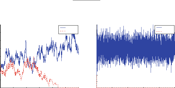
Figure 10.1 shows an SSA simulation of the model with these parameters. One

clonotype reaches extinction before t D 30, while the other clonotype remains and

ﬂuctuates about an average of approximately 32 cells for a very long time. At ﬁrst

we may think that the simulation has settled down to its stationary distribution but

this is not the case because extinction of both species is guaranteed in this model.

Thus we instead associate the long period with n>0shown in Fig. 10.1 with a

quasi-stationary distribution (QSD).

Here we give a simple argument to show that the simulation in Fig. 10.1 is in-

deed eventually absorbed. Note that Stirk et al. give a more sophisticated analysis

and establish that absorption is guaranteed in general. After extinction of one of the

clonotypes, we are left with a one-dimensional, inﬁnite state, birth-death process for

the remaining clonotype. There is an absorbing state at 0, and an irreducible class

f1;2;:::g, from which the absorbing state is accessible. Following standard nota-

tion and standard theory for birth-death processes [6], absorption with probability

one is equivalent to divergence of the series

iD1



:::



:::

00524681010 15 20 25 30

Time Time

Number

x 10

Type 2

Type 1

Type 2

Fig. 10.1 A simulation of the T cell clonotype populations

10 Stochastic Modelling of Two Competing Clonotypes 215

In the simulation in Fig. 10.1, after extinction of clonotype n

, the death rate is 

n and the function in (10.5)is

1  p

n C



i= i



;

for large n, so the birth rate 

 n.1=n/ D  for large n. With these observa-

tions it is straight-forward to show that the series diverges, for example by the nth

term test.

Although absorption is guaranteed, we can see from Fig.10.1 that the time to

extinction for both species is very large (at least t D 10

in this case). The length

of time that a clonotype spends in a QSD before being absorbed is identiﬁed as an

important issue and discussed in depth by Stirk et al. [5]. Bounds for the mean time

until absorption are given [5, Sect. 3]. Also, the work of N˚asell [24] is applied to this

process to ﬁnd the form of the QSD [5, Sect. 3.2.2]. Signiﬁcantly, it is shown that

clones with a smaller niche overlap last longer, because they face less competition

for survival stimuli. This mechanism drives the T cell repertoire towards greater

diversity and thus endows the immune system with a greater functional capacity for

recognizing a larger variety of foreign pathogens.

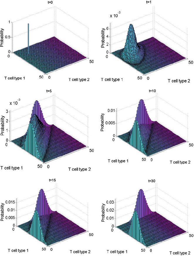
Figure 10.2 shows the evolution of the PDF associated with the model, computed

via a Krylov FSP algorithm for the solution of the Master Equation [20]. The PDF

starts as a delta distribution on the initial state, as seen in the ﬁgure labelled t D 0.

However, after a very short time, t D 1, it spreads out to resemble a Gaussian

distribution. By t D 5, it is trimodal. The middle peak then gradually disappears

so that by t D 30, only two of the original peaks remain. The remaining peaks

correspond to the QSD. Each peak corresponds to moderate levels of one T cell

clonotype and extinction of the other. The distribution is symmetric about the line

n D n

, reﬂecting the symmetry of this model.

Time-Dependent Propensity Functions

Thus far  has been a constant but Stirk et al. identify this as an issue for future

research and discuss the desire to consider it as a time-dependent parameter, be-

cause , which represents the strength of the stimulation that a T cell receives from

the relevant APPs, depends on the T cell repertoire, which changes with time as

some clones go extinct and new clones are released from the thymus [5]. It is well-

recognized that older individuals often have a weaker immune system, as evidenced

by the greater susceptibility of the aged to infection [2]. Very complicated processes

in immunobiology underly this aging effect but it may be due in part to a decline in

the strength of the birth rates. For example, there are limits to how many times that

a T cell may replicate, perhaps partly due to the shortening of the telomeres with

each replication [5, 25, 26], and the level of stimulation felt by a T cell clonotype

may decline with age [27]. This motivates us to consider a variation of the original

216 S. MacNamara and K. Burrage

Fig. 10.2 The initial delta distribution, at t D 0, on the initial state Œ10; 10, and the solution to

the Master Equation at times t D 1; 5; 10; 15; 30

model in which the birth rates decline with time. As Stirk et al. and others point out,

similar numbers of T cells are found in older and younger individuals [28]. Thus we

must bear in mind with what follows that we consider a reduction in birth rates for

some clonotypes but not all. Here we consider just two clonotypes, which is only a

small fraction of the total number of clones in the full T cell repertoire.

10 Stochastic Modelling of Two Competing Clonotypes 217

0 5 10 15 20 25 30

0.1

0.2

0.3

0.4

0.5

0.6

0.7

0.8

0.9

0 5 10 15 20 25 30

Time

φ (t)

Number

Type 1

Type 2

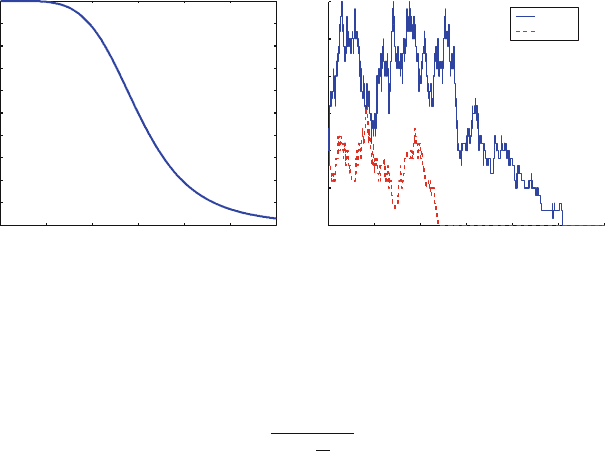
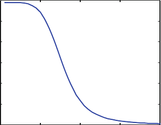
Fig. 10.3 (a) The time dependence of .t/ in (10.7). (b) A simulation of the T cell clonotype

populations, with the time-dependent propensities scaled as described near (10.7)

We represent time dependence by the hill function

.t/ D

1 C





; (10.7)

where K D 15 and m D 5. The function declines with time, with a steep sigmoidal

shape, as shown in Fig. 10.3a. We scale the propensities for the birth rates by .t/.

For this example, we replace  and 

in (10.6) with 60.t/. Thus at t D 0 the new

birth rates are the same as the old ones and remain similar for small values of t,but

for large values of t the new birth rates are much less than the old birth rates.

Figure 10.3b shows a simulation of the time-dependent process. This simulation

is obtained by a slight variation of the algorithm for the time-independent case [29].

The main subtlety here is in choosing the time step based on the exponential of

the integral of the propensity functions. We see the populations decline sharply at

t  15, corresponding to the decline in .t/. In contrast to the time-independent

case, both populations are extinct by t D 30.

Numerical Solution of the Time-Dependent Master Equation

Having considered a trajectory approach we now discuss complementary PDF ap-

proaches to the time-dependent case. Consider the system

.t/ D A.t/p.t /;

which is the same as in (10.1) except that here the matrix A.t/ is time-dependent.

In analogy with the constant-coefﬁcient case, we would like to ﬁnd a solution of the

form

p.t/ D exp



 .t/



p.0/:

218 S. MacNamara and K. Burrage

If, 8t;t

, A.t/ commutes with A.t

/,wehave

 .t/ D

A.s/ds:

In the constant-coefﬁcient case, the integral is  .t/ D tA, thus recovering (10.2)as

an important special case. Magnus [30] derived a formula for the general case:

 .t/ D

A.s

/ds



ŒA.s

/; A.s

/ds

ŒA.s

/; A.s

/; A.s

A.s

/; ŒA.s

/; A.s

/

C ::: (10.8)

Here the commutator ŒA; B is deﬁned as AB  BA . This inﬁnite series contin-

ues with higher order terms containing progressively higher order commutators and

higher order multiple integrals. Burrage has discussed the Magnus formula in the

context of stochastic differential equations [31]. It has been widely used for theo-

retical purposes but for numerical purposes, it is awkward to evaluate in this form.

For example, one may consider the approximation obtained by truncating the series

after suitably many terms. However, it is expensive to evaluate the many multiple in-

tegrals, and higher commutators, and it is not trivial to decide where to truncate the

series, or which terms should be selected to obtain the highest order approximation

for the least computational effort. Fortunately, in a series of papers on numerical

methods based on the Magnus formula, Iserles et al. [32] showed that the scheme

D A



; A

D A

;



N C1

h.A

C A

/ C

ŒA

; A

; (10.9)

p.t

N C1

/ D e



N C1

p.t

/; (10.10)

where t

N C1

D t

C h, is an order four approximation. Notice A

and A

are the

evaluation of the matrix at Gaussian quadrature points.

For this work, we implement this scheme in combination with a Krylov FSP

approach. The algorithm repeats two steps until the desired time point is reached:

ﬁrst, with a ﬁxed step size of h D 0:5,weformA

, A

and 

N C1

in (10.9);

then pass 

N C1

to the Krylov FSP solver and apply the update rule (10.10). We

refer to this procedure as the Magnus Krylov FSP algorithm. It is summarized in

Algorithm 2.

The algorithm requires the following inputs: the initial distribution, p.0/;the

time t

, at which the solution is required; and the matrix A representing the Markov

10 Stochastic Modelling of Two Competing Clonotypes 219

329 ALGORITHM 2: Magnus Krylov FSP.A; p.0/; t

;h)

330 t 0;

331 p.t/ p.0/;

332 while t<t

333 Compute A

, A

and 

N C1

in (10.9) with t

D t;

334 Compute e



N C1

p.t/ by Krylov FSP

335 p.t / e



N C1

p.t/ as in (10.10);

336 t t C h ;

337 end while

338 return p.t/;

chain. The initial distribution will often be a delta distribution on the initial state,

as in the examples in this paper. The algorithm also requires a way to evaluate the

matrix A.t/ at various time points. Although Algorithm 2 is described as if it re-

quires the full matrix A, in fact it does not need this. A function representing the

action of the matrix on a vector is sufﬁcient for a Krylov method. At any instant the

algorithm only requires a ﬁnite principal submatrix of the full matrix A. This ﬁnite

state projection can be dynamic so that it tracks most of the support of the distribu-

tion [18, 20]. The algorithm also requires a step size h and for this implementation

a ﬁxed step size of h D 0:5 was used. However this is a simpliﬁcation and in future

work adaptive step size strategies will be investigated.

Remarks. – In general Algorithm 2 expands the projection at each step as nec-

essary. However for the particular application in this paper we implemented a

simpliﬁed version of the algorithm. First, we truncate the state space to a size of

approximately 10;000. We use this same state space to form

A.t/ (8t). Note that

A.t/ is only an approximation to A.t/ but we will abuse notation and denote

both by A.t/.

– Due to the expansion around the initial state in whole numbers of steps of reach-

ability [20], the precise size of the state space employed by the algorithm is

10;076. Repeating the experiments with a smaller truncation size of 5;000 gives

results that are visually indistinguishable from the larger system.

– The sum of the conserved probability at each step is monitored and remains

>1 10

5

. In the constant coefﬁcient case this would guarantee accuracy, with

the computed solution being a lower bound on the true solution, within  D 10

5

in a component-wise sense. This suggests that the solution in our time-dependent

case is also very accurate. However, this is only a heuristic algorithm and a for-

mal analysis of the error behaviour is still to be considered.

– In the current implementation, at each step, A

, A

, ŒA

; A

 and ﬁnally  are

formed as sparse matrices and then  is passed to the Krylov solver, which em-

ploys an Arnoldi process together with an adaptive time step integration scheme.

The matrices A

, A

share the same sparsity pattern and are very sparse: the

density of non zeros is 5  10

4

. The commutator is about twice as dense, at

10

3

, but this is still very sparse. So the problem is well-suited to a Krylov

approach.

220 S. MacNamara and K. Burrage

– The solutions are computed within a few minutes. Matrices such as A

can be

formed in less than one second.

– In many applications A.t/ ! A

as t !1so that for sufﬁciently large t the

problem reduces to (10.1) with A replaced by the constant equilibrium matrix

. In these situations it is desirable to combine the Magnus Krylov FSP with

the standard Krylov FSP described in the previous section: initially, we employ

the Magnus method but after sufﬁciently large t is reached, we switch to the

cheaper, standard Krylov FSP. The successful application of this combination

requires a way to recognize when sufﬁciently large t has been reached. For the

application at hand, .t/ ! 0 for large t so we could employ this strategy for,

say t > 100, for example.

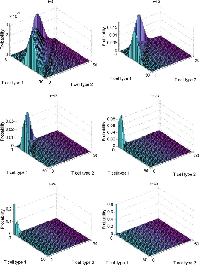
Figure 10.4 shows the evolution of the PDF in the time-dependent case. Ini-

tially, the distribution is similar to the time-independent case: compare, for example,

Fig. 10.4 at t D 5 with Fig. 10.2.However,att  8 the evolution starts to diverge

and by t D 13 the PDF is noticeably different. In particular we see the distribu-

tion gradually moving towards the origin at the snapshots in t D 13; 17; 23; 25,and

by t D 30 about 80% of the distribution is in the absorbing state. This is in con-

trast to the time-independent case for which the QSD lasts for a very long time. This

attenuation of the time spent in the QSD is signiﬁcant in understanding the immuno-

logical implications of the age-dependent case. As noted in above, diversity in the T

cell repertoire is maintained because clonotypes with a smaller niche overlap tend

to last longer because they face less competition for survival stimuli. However for

clonotype populations that show an age-dependent decline in  as in (10.7), the QSD

may not last very long even if the clonotype has a small niche overlap. This results

in an abnormal loss of diversity from the T cell repertoire. corresponding decrease

in the functional capacity of the immune system to recognize foreign epitopes.

The Mean Time to Extinction of Both Clonotypes

In this section we quantify how the survival time of a clonotype depends on the

time-dependence of the birth-rates. Assuming that the process begins in the quasi-

stationary distribution, the mean time until absorption is given by 1=

,where

the decay parameter associated with the Markov chain. For many applications, after

a brief initial transient the process is approximately in the QSD so this is a reason-

able assumption. The theory of the decay parameter and QSDs is presented in [33].

Thus we use 1=

as an indication of the survival time of a clonotype. For the bi-

variate clonotype model, we compute the eigenvalue, , with smallest magnitude, of

the matrix A

.HereA

is same as the FSP (10.3), except that the absorbing state

has also been removed. One way to compute  is to use the inverse power method,

or to call the MATLAB sparse eigenvalue routine, eigs.A

;1;0/. We approximate

the decay parameter by 

. Note that there are some technical issues with

this approximation for inﬁnite models [33–36]. Although the clonotype models are

10 Stochastic Modelling of Two Competing Clonotypes 221

Fig. 10.4 The solution to the ME at t D 5; 13; 17; 23; 25; 30 in the time-dependent case

inﬁnite this is because bounds are not known and may be large. Real applications

will have ﬁnite numbers of clonotypes so it is reasonable to focus on the ﬁnite case.

Figure 10.5 shows the change in the mean time to absorption, from the QSD, as a

function of time. It can be seen that the time-dependence resembles that of the time-

dependent birth rates in Fig. 10.3a, although on a log scale. At t D 0, the average

222 S. MacNamara and K. Burrage

0 10 20 30 40

log(1/λ

)

Fig. 10.5 The mean time until extinction of both clonotypes in the two-dimensional model

lifetime of a clonotype is 10

but at t D 20 the lifetime is only 10

. This shows

that the simulation in Fig. 10.1 would probably not go extinct until 10

. Also, this

shows that the reduction in the birth rates over time, by about an order of magnitude,

leads to a much larger effect on the life expectancy of a clonotype, which decreases

by several orders of magnitude.

Discussion

This work has focused on the implications of a particular functional form of the

time-dependence for diversity maintenance but future work will consider the signif-

icance of different functional forms for .t/. Furthermore it would be interesting to

explore parameter space and models that have more clonotypes. For example this

work focused on the case that   1 but it would be interesting to relax this assump-

tion and consider the model with appropriate approximations to the birth rates. We

identify a number of important areas for reﬁning the numerical methods described

here:

– Generalizing the error analysis of the Krylov FSP approximation to:

 A time-dependent matrix

 A combination of the Krylov FSP with the order 4 approximation

– Employing adaptive time-steps in the Magnus Krylov FSP integrator.

– Identifying a more sophisticated embedding of the Magnus formula in the

Krylov methods, for improved computational efﬁciency. For example, as a

Krylov method, only a function that returns the action of  on a given vector, v,

is required, so we do not need to form the matrix, or the commutator in (10.9).

Instead, one possibility is to employ the following scheme. First form the vectors,

D A

v; w

D A

v; w

D A

; w

D A

;