Muga G. Time in Quantum Mechanics - Vol. 2
Подождите немного. Документ загружается.


244 J. Martorell et al.
In this chapter we avoid unnecessary repetition of thoroughly reviewed material,
although some well-known topics will be also briefly outlined for completeness.
These include the Paley–Wiener theorem, see below, and a brief reminder of basic
results of the discrete–continuum model in Sect. 9.2. We shall rather concentrate on
some recent results and potential scattering. Decay of a single particle from a trap
will be the main physical system under discussion in Sects. 9.2 (devoted to sim-
ple models) and 9.3 (on explicit decay laws depending on the long-range potential
tail). Section 9.4 reviews different physical interpretations that have been given to
post-exponential phenomena, and Sect. 9.5 the difficult route toward experimental
observation. In the remainder of this section we introduce the basic and seminal
work by Khalfin, with only a brief account of what preceded him.
9.1.3 Early Work and Paley–Wiener Theorem
Following the theories of Gamow, and Weisskopf and Wigner, Hellund [56] ana-
lyzed the decay of resonance radiation and showed that decay could not be exactly
exponential. He also noted that it should be slower at long times. Later on, H
¨
ohler,
going beyond the simplifications of the Weisskopf–Wigner model, obtained a power
law for long times [58]; see also [114] for an early study of nonexponential alpha-
decay.
Khalfin [65] discovered a very general result: the long-time decay for Hamil-
tonians with spectra bounded from below is slower than exponential. Here is the
argument: Consider a system described by a time-independent Hamiltonian, H,
initially in a normalized nonstationary state |Ψ
0
. The survival amplitude of that
state is defined to be the overlap of the initial state with the state at time t and is the
expectation value of the time evolution operator
A(t) =Ψ
0
|exp(−iHt/)|Ψ
0
. (9.2)
The survival probability, sometimes called the “nondecay probability” [38], is
1
1
The survival probability is sometimes criticized as a measure of decay. For example, in a simple
half-scattering problem with a particle located initially in a trapping potential, it may be difficult to
measure. Some decay analyses therefore discuss other quantities, such as the nonescape probability
from a region of space [43, 92], the probability density at chosen points of space [89, 88, 133], the
flux [94, 95, 141], the arrival time [2]. For initially localized wave packets, there is no major
discrepancy between survival probability and the nonescape probability. A claim to the contrary
for long-time decay in [43] was criticized [89, 9, 136, 135] and confirmed later to be the result
of a nonconverged computation [45]. Examination of densities, fluxes, or arrival time distributions
may be interesting since a new variable is introduced but at the price of losing the simplicity and
uniqueness of the survival probability.
A property of the survival amplitude not necessarily shared by other decay measures is its
“stationarity.” To formulate it we require a more precise notation: Let P(t, t
0
) =|ψ(t
0
)|ψ(t)|
2
be the survival probability at time t of the state ψ(t
0
). It then follows from the hermiticity of H
that P(t, t
0
) = P(t + t
, t
0
+ t
), in other words, for a given wave packet the survival amplitude

9 Quantum Post-exponential Decay 245
P(t) =|A(t)|
2
. (9.3)
The stationary states, H|Φ
E,λ
=E|Φ
E,λ
(where λ denotes any other quantum
numbers comprising a complete set of commuting observables), determine a basis.
We assume that the Hamiltonian has only a continuous spectrum or at least that the
discrete states of H are orthogonal to Ψ
0
. Further, we assume that the spectrum is
bounded from below: E
m
< E < ∞. The completeness relation is then
λ
∞
E
m
dE |Φ
E,λ
Φ
E,λ
|=1 , (9.4)
which gives
A(t) =
∞
E
m
dE ˜ω(E)e
−iEt/
, where
˜ω(E) =
λ
|Φ
E,λ
|Ψ
0
|
2
(9.5)
is called the “energy density” of the quasi-stationary state. It is then natural to define
ω(E) =
˜ω(E) , E ≥ E
m
0 , E < E
m
(9.6)
and express the survival amplitude as the Fourier transform of the energy density
[70],
A(t) =
∞
−∞
dEω(E)e
−iEt/
. (9.7)
Khalfin showed that when ω(E) is so bounded from below, the Paley–Wiener theo-
rem [111] requires that
∞
−∞
dt
ln |A(t)|
1 + t
2
< ∞ . (9.8)
For this integral to converge as t →∞, the numerator must grow no faster than
∝ t
2−a
with a > 1. This clearly rules out exponential decay at sufficiently long
times. Assuming such a bound,
P(t) ≥ Ae
−β|t|
q
, (9.9)
P(t
2
, t
1
) is a function only of the time difference t
2
− t
1
. This may seem strange at first, but note
that usually only the case in which the initial wave packet is localized in a region of space is of
physical significance in a decay process.

246 J. Martorell et al.
with A > 0, β>0, and q < 1. An alternative proof, avoiding use of the Paley–
Wiener theorem, has been given by Hack [54].
9.1.3.1 Decay at Post-exponential Times with Energy Integrals
Given an explicit expression for the energy density, to find analytic approximations
for the post-exponential contribution to P(t), one may replace the integration path in
Eq. (9.5) by a contour integral in the complex plane [38, 67, 109]. For convenience,
we place the origin of energy at threshold, E
m
= 0, and choose a closed contour
consisting of the positive real energy axis, a quarter circle of infinite radius running
clockwise from the positive real axis to the negative imaginary axis, and continuing
to the origin. Under very general conditions, integration along the circular arc gives
a vanishing contribution. Then,
A(t) =
∞
0
dE ω(E)e
−iEt/
=
5
dE ω(E)e
−iEt/
+
−i∞
0
dE ω(E)e
−iEt/
≡ A
p
(t) + A
v
(t) , (9.10)
where we have analytically continued ω(E) into the lower half of the complex plane.
Depending on the analytic structure of ω(E), this may or may not be a simple task.
The contour integral A
p
(t)is2πi times the sum of residues of poles in the fourth
quadrant. These poles correspond to exponentially decaying terms.
The integral along the imaginary axis, A
v
(t), gives the dominant contribution to
the decay at long times. We write the variable of integration as
˜
E = iE to obtain
A
v
(t) = i
∞
0
d
˜
E e
−
˜
Et/
ω(−i
˜
E) . (9.11)
The exponential term becomes negligible after many lifetimes, say when t τ =
/Γ , with Γ the width of the lowest lying resonance in ω(E). At such times t,
the exponential in Eq. (9.11) restricts the range of significant contributions to the
integral to values of
˜
E Γ , which means to energies close to threshold.
A simple example is a pure Lorentzian energy density,
ω
L
(E) =
Γ/(2π )
(E − E
R
)
2
+Γ
2
/4
. (9.12)
In Sect. 9.2.2 we show how this appears, under suitable approximations, for a dis-
crete state coupled to a continuum. (See also [38] pp. 604–606 for a similar but
more elaborate model.) This energy density has a pole at E = E
R
− iΓ/2, giving
the exponential decay contribution
A
p
(t) = e
−iE
R
t/
e
−Γ t/2
. (9.13)
9 Quantum Post-exponential Decay 247
In addition, when t →∞,
A
v
(t) = i
Γ
2π
∞
0
d
˜
E
exp(−
˜
Et/)
(−i
˜
E − E
R
)
2
+Γ
2
/4
i
Γ
2π
E
2
R
+Γ
2
/4
1
t
+O
1
t
2
, (9.14)
where in the second line we have set
˜
E = 0 in the denominator to evaluate the
integral. This model therefore predicts that asymptotically, when the exponential
term in Eq. (9.13) becomes negligible, P(t) |A
v
(t)|
2
∝ t
−2
.
Notice that due to the phase −E
R
t/ in A
p
(t), in the range of times where the
two contributions are of similar magnitude, interference oscillations are expected to
occur. For a complete analysis of the decay for a more realistic truncated Lorentzian,
including an exact expression for A(t) and additional terms in the expansion of
A
v
(t), see [130].
Suppose now that E
R
decreases toward threshold at E
m
= 0. As the pole moves
toward the negative imaginary axis it increases the value of A
v
(t), eventually making
it comparable to A
p
(t). In the limit E
R
= 0 obviously the above decomposition is
invalid, implying that the decay ceases to be exponential. This is known as small
Q-value decay. For a more complete theoretical analysis of this situation and some
particular model examples, see [63]. According to that analysis, small Q-value
decay becomes noticeable when Q ≡ E
R
− E
m
≤ Γ/2.
The simplicity of the above model has made it popular in discussions of expo-
nential decay. Jakobovits et al. [62] have shown that the steepest descent method
applied directly to Eq. (9.5) also leads to exponential decay and shows that any
corrections to it should usually be small.
Although useful as an illustration, Eq. (9.12) is far from being a realistic model
for the energy density, in particular for the asymptotic law, since the Lorentzian
form is generally not valid near threshold.
9.2 Simple Models and Examples
To fully appreciate post-exponential decay it is useful to understand first why expo-
nential decay should be expected at all in a quantum system, even if only approxi-
mately, or over some limited time interval. The Gamow and Weisskopf–Wigner the-
ories provide a clue, but a fresh look at the survival amplitude, Eq. (9.2), could raise
doubts about the robustness of exponential decay, since a properly chosen initial
state Ψ (0) and energy density are amenable to an almost arbitrary decay law [46].
This puzzle is perhaps easier to understand in discrete–continuum decay models
[113] (see below for an elementary illustration), but it has also been discussed in the
context of scattering processes, e.g., in [47, 38]. If the initial preparation involves
localization, the initial wave function will overlap prominently with scattering func-
tions in certain regions of the energy spectrum, close to resonant poles, since they

248 J. Martorell et al.
are more localized in the interaction region than ordinary, non-resonant waves. Con-
tributions from broad resonances will decay faster, whereas for a narrow resonance it
is the analytical structure of the pole rather than the complete state amplitude, which
dominates the behavior, leading in practice to an “effective” Lorentzian energy
density and through it to exponential decay.
9.2.1 Discrete State Embedded in a Continuum
Let us assume a simple Hamiltonian of the form
H = E
φ
|φφ|+
dEE|EE|+
dEW(E) |φE|+h.c.
. (9.15)
This is a typical nondegenerate single-channel Hamiltonian model which neglects
continuum–continuum interactions. Other versions are due to Fano [34], Anderson
[1], Lee [72], and Friedrichs [40] and have been successfully applied to study, for
example, autoionization, photon emission, or cavities coupled to waveguides. The
dynamics can be solved in several ways, using coupled differential equations for the
time-dependent amplitudes and Laplace transforms, or finding the eigenstates with
Feshbach’s (P, Q) projector formalism [35], which allows separation of the inner
(discrete) and outer (continuum) spaces and provides explicit expressions ready
for exact calculation or phenomenological approaches. For modern treatments with
emphasis on decay, see [24, 108]. Writing the eigenvector as [34, 24]
|Φ
E
=|φφ|Φ
E
+
dE
|E
E
|Φ
E
, (9.16)
the coefficients for the discrete state are determined to be, using Laplace transform
techniques or the projector P, Q formalism,
|φ|Φ
E
|
2
=
|W(E)|
2
[E − E
φ
− F(E)]
2
+π
2
|W(E)|
4
, (9.17)
where
F(E) = P
dE
|W(E
)|
2
/(E − E
) . (9.18)
If W (E) → W is energy independent, which is the essence of the Weisskopf–
Wigner approximation, and if the range of integration is extended from −∞ to ∞,
then F(E) = 0 and |φ|Φ
E
|
2
becomes a Lorentzian,
|φ|Φ
E
|
2
=
Γ/2π
(E − E
φ
)
2
+Γ
2
/4
, (9.19)
9 Quantum Post-exponential Decay 249
with Γ = 2π|W|
2
. Then, if the initial state is precisely φ, the energy density is
a Lorentzian (Breit–Wigner form) and as we have shown in Sect. 9.1, its survival
probability has an exponential component
P(t) = e
−Γ t/
. (9.20)
For weak coupling of bound state to continuum, the resonance is long-lived and
its width is small, so that the constant-W approximation holds quite well. How-
ever, there is a fundamental physical limit to its validity, namely the existence of
the energy threshold. If the resonance energy is close to threshold, this effect will
be more noticeable, or even dominant, to the point of making the decay totally
nonexponential [63, 42].
9.2.2 Simple Models Set in the Momentum Plane
Many decay models and in particular potential scattering models are treated in the
complex momentum plane. The basic “mathematical” reason for exponential decay
is easily seen to be the presence of a complex pole in the fourth quadrant of the
momentum complex plane (second Riemann sheet of the energy plane), which,
through its exponentially decaying residue, dominates the dynamics for some time.
A simple analytical example of the deviation from exponentiality follows from the
integral expression for the survival amplitude,
A(t) =Ψ
0
|e
−iHt/
|Ψ
0
=
i
2π
C
dq e
−izt/
I(q) , (9.21)
where
I(q) =
q
m
Ψ
0
|
1
z − H
|Ψ
0
, (9.22)
z = q
2
/2m, and the contour C goes from −∞ to ∞ passing above all singularities
in the complex momentum plane q. One-dimensional motion of a particle of mass
m is assumed. Consider now a pole expansion of the form I(q) =
a
k
/(q − q
k
)
[90, 45]. Since each term can be analyzed separately and combined linearly later,
we concentrate on a single pole, I (q) = a
r
/(q − q
r
), with q
r
assumed to lie above
the diagonal of the fourth quadrant and below the real axis. The integral is easily
evaluated by deforming the contour to run diagonally across the second and fourth
quadrants and picking up a small circle surrounding the pole. This gives
A(t) =
1
2
a
r
w(−u
r
) = a
r
exp(−u
2
r
) −
1
2
sgn[Im(u
r
)]w[sgn[Im(u
r
)]u
r
]
,
(9.23)
where
250 J. Martorell et al.
u
r
= q
r
/ f, f = (1 −i)(m/t)
1/2
, (9.24)
and w(z) = exp(−z
2
)erfc(−iz).
2
We have used the relation
w(−z) = 2e
−z
2
−w(z) . (9.25)
Equation (9.23) is particularly suitable for analyzing exponential decay, explicitly
given by the pole, and its deviation, given by the line integral along the diagonal,
evaluated as a w-function. The function w(z) has the asymptotic expansion
w(z) ∼
i
√
π z
1 +
1
2z
2
+...
, (9.26)
which, for long times, leads to a 1/t
1/2
behavior.
However, an I (q) with a single pole would be incompatible with time-reversal
symmetry A(t) = A(−t)
∗
. The minimal model compatible with time-reversal must
include, in addition to the resonance at q
r
, the antiresonance pole at −q
∗
r
,
I(q) =
a
r
q − q
r
+
a
∗
r
q + q
∗
r
, (9.27)
with a
r
= 1 + iIm q
r
/Re q
r
[44]. The contour integral along the diagonal which
defines the u variable does not enclose this antiresonance pole, so it does not provide
an exponentially decaying term but an additional contribution (the w(u
r
)-function)
that is significant only at short and long times [44]. In particular, it cancels exactly
the asymptotic t
−1/2
decay from the resonance pole. However, the second terms in
Eq. (9.26) do not cancel, resulting in a leading t
−3/2
behavior for A(t).
So far this is a pure decay model rather than a Hamiltonian model; for an applica-
tion see, e.g., [92]; but Hamiltonian realizations are possible. The separable potential
considered in [90, 88, 89] leads to three core (state-independent) poles, two of them
forming a resonance/antiresonance pair. Even closer to the minimal decay model is
the delta-shell potential, discussed is the next section, when only the lowest reso-
nance is excited and higher resonances can be neglected. Then it is exactly described
by Eq. (9.27).
A general and useful result, independent of the assumed pole expansion, follows
from noting that if the resolvent matrix element in Eq. (9.21) admits a series expan-
sion, c
0
+c
1
q +c
2
q
2
+..., the leading term in the asymptotic formula, obtained by
term by term integration, is
A(t) ∼
1
m
√
2πi
c
1
m
t
3/2
, (9.28)
2
%
∞
−∞
e
−u
2
u−z
= iπ sgn[Im(z)] w{z sgn[Im(z)]}.

9 Quantum Post-exponential Decay 251
c
0
does not contribute by symmetry. For explicit examples of this, see [89], where
a similar analysis is performed for the propagator and probability density. Further
details are given in Sect. 9.4.2.
9.2.3 Exponential Decay as a Boundary Condition
Torrontegui et al. [133] have recently proposed a minimal, solvable 1D “source”
model based on imposing an exponentially decaying amplitude for all times at one
point in space (x = 0). This provides an economical approach to mimic analyti-
cally the wave function due to an exponentially decaying system with a long-lived
resonance, while avoiding a detailed description of the interaction region where the
decaying system is prepared. Deviations from exponential decay are observed in the
probability density at x > 0.
9.2.4 One-Dimensional Well-Barrier Model of Confining Potential
One of the simplest 1D models of a decaying particle with a full description of
the dynamics, including the preparation region, consists of a flat well surrounded
by equal square barriers: in units = 2m = 1, we write V(x) =−V
0
when −a
< x < a; V(x) = V
b
when a < |x| < d and V(x) = 0 when |x| > d.The
initial state is chosen symmetric: Ψ
0
(x) = 1/
√
a cos(π x/(2a) Θ(a −|x|), and the
continuum wave functions are
Ψ (x; E) =
⎧
⎨
⎩
N cos k
I
x , |x| < a
A
b
e
κx
+ B
b
e
−κx
, a < x < d
1
√
2πk
cos[kx − δ(k)] , d < x
(9.29)
for x > 0, while Ψ (−x) = Ψ (x). Here k
2
= E, k
I
=
/
k
2
+V
0
, and κ =
/
V
b
−k
2
. The normalization of the outer part is determined by the condition
∞
−∞
dx Ψ (x; E) Ψ (x; E
) = δ(E − E
), (9.30)
which leads to
N
2
=
1
2πk
cosh
2
(κb) +
κ
2
k
2
I
sinh
2
(κb)
cos
2
(kd −δ(k))
+
k
2
κ
2
sinh
2
(κb) +
κ
2
k
2
I
cosh
2
(κb)
sin
2
(kd −δ(k))
+2
k
κ
sinh(κb) cosh(κb)sin(kd −δ(k)) cos(kd −δ(k))
1 +
κ
2
k
2
I
.
(9.31)
252 J. Martorell et al.
In terms of these, the energy density is
ω(E) ≡|Ψ
0
|Ψ (E)|
2
=
N
1
√
a
a
−a
dx cos k
I
x cos
π
x
2a
!
2
=
N
2
a
π/a cos k
I
a
k
2
I
−π
2
/(4a
2
)
2
. (9.32)
The asymptotic behavior, when E → 0, is easily found to be ω(E) ∝ k
−1
. Applying
Eq. (9.11) one finds
A
v
(t) ∝ t
−3/2
, P(t) ∝ t
−3
. (9.33)
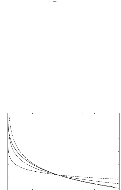
Figure 9.4 is drawn for the parameters: V
0
= 0.5, V
b
= 1.8, a = 1.0, and d = 1.4.
The exact survival probability is compared to some alternative asymptotic forms of
P(t) and shows that indeed the asymptotic time dependence is that of Eq. (9.33).
1e-06
1e-05
1e-04
1e-03
1e-02
1e-01
1
200 400 600 800 1000 1200 1400 1600
Survival probability
time
Fig. 9.4 Survival probability, P(t) vs. time for the 1D-confining potential described in the text.
Continuous line: exact solution of the TDSE. The three dashed lines correspond to asymptotic
decays proportional to 1/t, 1/t
2
,and1/t
3
. The proportionality constants have been adjusted to
reproduce the exact P(t = 800)
9.3 Three-Dimensional Models of a Particle Escaping
from a Confining Potential
In this section, we directly obtain the energy densities and asymptotic decay profile
for specific and increasingly realistic potential forms.

9 Quantum Post-exponential Decay 253
9.3.1 The Delta-Shell Model
Winter [141] gave the first explicit example of the validity of Khalfin’s prediction.
He studied 1D motion on the half-line x ≥ 0, with a delta barrier at x = a and zero
potential elsewhere. He took the initial wave function to be the ground state of an
infinite well, Ψ
0
(x, t = 0) =
√
2/a sin(π x/a) Θ(a − x), and showed that the mean
momentum and the current at long times deviated from those of pure exponential
decay, making a few analytical approximations. Recently the same problem has been
re-analyzed by Dicus et al. [22] and indeed they find that the survival probability
deviates from exponential at long times.
Winter’s model and its variants have been applied on many subsequent occa-
sions, for example, to study the effect of a distant detector (by adding an absorptive
potential) [18], anomalous decay from a flat initial state [31], resonant state expan-
sions [45], initial state reconstruction [92], or the relevance of the non-Hermitian
Hamiltonian concept (associated with a projector formalism for internal and external
regions of space) in potential scattering [125]. In [125] the model was extended to a
chain of delta functions to study overlapping resonances.
Del Campo et al. [17] have also generalized the model for a Tonks–Girardeau gas
of N bosons with strongly repulsive contact interactions as well as spinless fermions
with strongly attractive contact interactions, and studied the long-time asymptotics
and some new effects in the few-body decay of these systems.
9.3.2 Well-Behaved Short-Range Potentials
Spherically symmetric potentials V(r) in three dimensions conserve angular momen-
tum. One can separate the wave function into partial waves or channels of given
angular momentum . For each partial wave, the radial Schr
¨
odinger equation is
d
2
w
dr
2
−
( + 1)
r
2
w
+[k
2
−V(r)]w
= 0 , (9.34)
where V(r) = (2m/
2
)V (r), k
2
= (2m/
2
)E, and w
(k, r)/r is the radial wave
function in channel . From the low-energy behavior of w
one can extract the
threshold behavior of the energy density ω(E) and from there, the time dependence
of the post-exponential survival probability. For so-called well-behaved potentials
this is a standard exercise in potential scattering theory [131]. These potentials
decrease as 1/r
3
or faster when r →∞and are less singular than 1/r
3/2
when
r → 0+. We will now summarize the derivation given in [80]. We work with
solutions normalized as
∞
0
dr w
(k
, r)
∗
w
(k, r) = δ(k
−k) (9.35)
and obeying the boundary condition w
(k, 0) = 0. At large distance