Muga G. Time in Quantum Mechanics

Подождите немного. Документ загружается.

8 Experiments on Quantum Transport of Ultra-Cold Atoms in Optical Potentials 223

fluorescence [arb. units]

position [mm]

(a)

(b)

–6 –4 –2 0 2

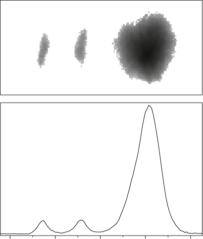
Fig. 8.9 Part (a) shows a ﬂuorescence image from an atomic distribution acquired after a time of

ballistic expansion. Part (b) shows the distribution integrated in the vertical direction. The large

peak on the right is the part of the atomic cloud that was not trapped during the initial acceleration.

The center peak indicates the atoms that were initially trapped in the ﬁrst band but were driven

out by the modulation. The left peak corresponds to atoms that remained trapped during the entire

sequence. The survival probability is the area under the left peak normalized by the sum of the

areas under the left and center peak

trapped in the ﬁrst band, which was obtained by summing the contributions of class

(2) and class (3).

To observe the temporal evolution of the fundamental band population, we

repeated the sequence in Fig. 8.8 for various modulation durations, holding the

probe frequency ν

and amplitude m ﬁxed. These studies resulted in the observa-

tion of Rabi oscillations between Bloch bands [13]. For large amplitudes of the

modulation, we observed a dynamical suppression of the band structure, effectively

turning off Bloch tunneling [28].

To obtain a spectrum of the Wannier–Stark states, we applied the modulation

during a period of constant acceleration and repeated the sequence for various probe

modulation frequencies, holding the modulation amplitude m and the duration ﬁxed.

Figure 8.10 shows three measured spectra for the accelerations of 947, 1260, and

1680 m/s

, which correspond to the Bloch frequencies ω

/2π = 16.0, 21.4, and

28.5 kHz, respectively. The spectra were obtained at a ﬁxed well depth of V

/h =

91.6 kHz and a ﬁxed probe modulation amplitude of m = 0.05. For a well depth

224 M.C. Fischer and M.G. Raizen

40 60 80 100 120 140

160

(c)

probe frequency [kHz]

(b)

survival probability

0.2

0.3

0.4

0.5

0.6

0.7

0.8

0.3

0.4

0.5

0.6

0.7

0.3

0.4

0.5

(a)

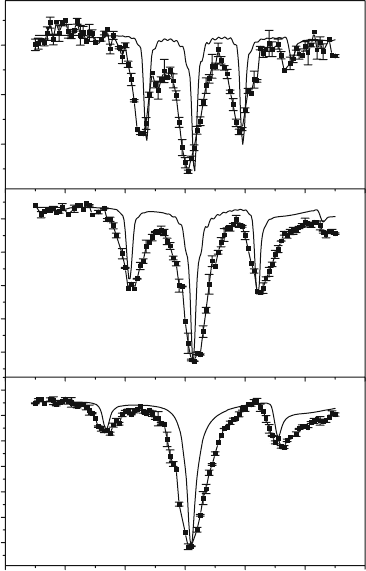
Fig. 8.10 Wannier–Stark ladder resonances for a well depth of V

/h = 91.6 kHz and accelera-

tions of (a) 947 m/s

,(b) 1260 m/s

,and(c) 1680 m/s

, which correspond to the Bloch frequencies

/2π = 16.0, 21.4, and 28.5 kHz, respectively. For the chosen well depth, the average band

spacing is

/h = 104 kHz which is in good agreement with the location of the central resonance.

The points are connected by thin solid lines for clarity. The thick solid lines show the results of

American Physical Society

of V

/h = 91.6 kHz, the average band spacing is

/h = 104 kHz, which is in

good agreement with the location of the central resonance in the three spectra of

Fig. 8.10.

Also shown in Fig. 8.10 is the result of a numerical integration of the time-

dependent Schr

odinger equation using the experimental parameters. We believe

that phase noise in the interaction beams prevented the survival probability from

reaching unity, when the probe was far from resonance, and reduced the depth

of the spectral features by a constant factor. For this reason, the y-values of the

theory curves were shifted and scaled to match the baseline and amplitude of the

central resonance. In addition, the value for the probe modulation amplitude m was

8 Experiments on Quantum Transport of Ultra-Cold Atoms in Optical Potentials 225

adjusted in the numerical simulations from 0.05 to 0.035 to reproduce the relative

peak heights.

The spectral width of the resonances is fundamentally determined by the ﬁnite

lifetime of the Wannier–Stark states due to tunneling. However, a number of exper-

imental mechanisms (e.g., phase noise in the standing wave beams, variations in the

well depth, or the ﬁnite transverse extent of the optical potential) contributed to the

measured width being substantially broader than that predicted by the simulations.

8.5 Quantum Tunneling

In the previous section we studied the spectral features of Bloch states and Wannier–

Stark states by driving transitions between those states. These inter-band transitions

were imposed externally by a modulation of the potential. Without modulation the

band index was conserved. The accelerations that transported the atoms through

reciprocal space were small enough to preserve the validity of the semiclassical

equations of motion. In this section we investigate the effect of a large accelera-

tion of the optical potential. In this case the semiclassical equations no longer hold

and inter-band tunneling can occur. The atoms can leave the trapping potential via

tunneling into the continuum of free states. The system is therefore unstable and

the number of trapped atoms decays with time. By adjusting the acceleration the

stability of the system can be altered dynamically and the decay rates vary over

a wide range. In this system, short-time deviations from the universal exponential

decay law are observed [42]. In addition, we study the fundamental effects of mea-

surements on the decay rate and report on the ﬁrst observation of the quantum Zeno

and anti-Zeno effects in an unstable system [12].

8.5.1 Classical Limit

As derived in Sect. 8.4, atoms in an accelerated standing wave are subject to a

potential

V (x) = V

cos(2k

x) + Max . (8.33)

This potential is stated in the reference frame accelerated with the potential as given

in Eq. (8.27). For a small enough acceleration a particle can be classically trapped

within the wells of this “washboard” potential. In this case the particle will accel-

erate along with the potential. For a larger acceleration the potential wells become

increasingly asymmetric up to a point where the particle is no longer conﬁned by

the potential. The critical acceleration a

c,class

, for which the potential loses its abil-

ity to conﬁne the particle, can be found by solving for extrema of the potential in

Eq. (8.33), which only exists for

|a| < a

c,class

. (8.34)

226 M.C. Fischer and M.G. Raizen

For accelerations smaller than a

c,class

the particle gets accelerated along with the

potential whereas for larger accelerations there are no local potential minima.

8.5.2 Landau–Zener Tunneling

8.5.2.1 Tunneling Rates

In this section we provide a short description of the Landau–Zener tunneling process

based on diabatic transitions in momentum space [35, 44]. An alternative description

can be derived in the position representation [26, 45]. As a starting point we consider

the semiclassical equations of motion describing the time evolution of the quasi-

momentum in reciprocal space. In order to allow for inter-band transitions, we must

now abandon the condition that the band index be a constant of motion. The shape

of the Bloch bands and the time evolution equation for the quasi-momentum are still

assumed to be valid. The stationary periodic potential causes the free particle energy

levels to undergo a level repulsion. This shift is most pronounced at the edges of the

Brillouin zone. A particle approaching the avoided level crossing might not be able

to follow the dispersion curve adiabatically, in which case it continues its motion

and diabatically changes levels across the energy gap. In 1932 Zener derived an

expression for the probability P of diabatic transfer between two repelled levels [44]

P = exp

−

2

(ε

−ε

)

, (8.35)

where E

is the minimum energy separation of the perturbed levels and ε

1,2

are

the unperturbed energy eigenvalues of level 1 and 2, respectively. In our case the

unperturbed energy curve is simply the free particle kinetic energy dispersion E

/2M. Using the semiclassical equation of motion for the quasi-momentum, we

obtain for the probability of transfer

P = e

−a

, (8.36)

where the critical acceleration a

is given by

n 

. (8.37)

We let N denote the number of particles populating the lowest band within the ﬁrst

Brillouin zone. The rate of atoms crossing the band gap is equal to the rate of atoms

approaching the transition region times the probability of tunneling if we assume the

band to be uniformly populated. We obtain an exponential decay of the population

N in the band under consideration as

N = N

−Γ

, (8.38)

8 Experiments on Quantum Transport of Ultra-Cold Atoms in Optical Potentials 227

with the Landau–Zener (LZ) decay rate Γ

given by

−a

. (8.39)

Experimental studies of the tunneling rates out of the lowest band were performed

in our group and the decay rates were compared to the Landau–Zener prediction [3,

27].

8.5.2.2 Deviations from Landau–Zener Tunneling

The expression for the LZ tunneling rate derived above is based on a single transit

of the atom through the region of an avoided crossing. However, for small tunneling

probability the atom can undergo Bloch oscillations within a given band, leading to

multiple passes through the Brillouin zone. The tunneling amplitudes can interfere

constructively or destructively depending on the rate at which the atom traverses

the Brillouin zone. This mechanism is responsible for the formation of tunneling

resonances. For small accelerations the tunneling rate is small and the atoms can

perform many Bloch oscillations before leaving the band. Therefore large deviations

from the Landau–Zener prediction for the tunneling rate are to be expected. For a

larger acceleration the atom leaves the band quickly and the interference effects are

less pronounced. For those cases the LZ prediction is a good approximation for the

actual tunneling rate. These statements are in agreement with the observed tunneling

rates [3, 27].

8.5.3 Non-exponential Decay

8.5.3.1 Theoretical Description

An exponential decay law is the universal hallmark of unstable systems and is

observed in all ﬁelds of science. This law is not, however, fully consistent with

quantum mechanics and deviations from exponential decay have been predicted for

short as well as long times [20, 43, 14]. In 1957 Khalﬁn showed that if H has a

spectrum bounded from below, the survival probability is not a pure exponential but

rather of the form

lim

t→∞

P(t) ≈ exp(−ct

) q < 1, c > 0 . (8.40)

Later Winter examined the time evolution in a simple barrier-penetration prob-

lem [43]. He showed that the survival probability begins with a non-exponential,

oscillatory behavior. Only after this initial time does the system start to evolve

according to the usual exponential decay of an unstable system. Finally, at very long

times, it decays like an inverse power of the time. The initial non-exponential decay

behavior is related to the fact that the coupling between the decaying system and the

228 M.C. Fischer and M.G. Raizen

reservoir is reversible for short enough times. Moreover, for these short times, the

decayed and undecayed states are not yet resolvable, even in principle.

A simple argument will illustrate this point. We assume that the system is initially

in the undecayed state |Ψ

 at t = 0, and that the state evolves under the action of

the Hamiltonian H,

|Ψ (t)=e

−iHt/

|Ψ

=A(t)|Ψ

+|Φ(t) , (8.41)

where A(t) is the probability amplitude for remaining in the undecayed state and

the state |Φ(t) denotes the decayed state with Ψ

|Φ(t)=0. The probability of

survival P in the undecayed state is therefore P(t) =|A(t)|

. Acting with the time

evolution operator e

−iH(t+t



)/

on the state |Ψ

 yields

A(t + t



) = A(t)A(t



) +Ψ

−iHt



/

|Φ(t) . (8.42)

If it were not for the last term, the equation above would generate the characteristic

exponential decay law of an unstable system. However, the term under consideration

describes the possibility for the decayed state |Φ(t) to re-form the initial state |Ψ



under the time evolution operator for time t



For very short times we can make a general prediction about the time evolution of

the survival probability P. Given that the mean energy of the decaying state is ﬁnite

and that H has a spectrum that is bounded from below, one can show following the

arguments of Fonda et al. [14] that

dP(t)



t→0

= 0 . (8.43)

As outlined by Grotz and Klapdor [18] we can expand A(t) in a power series

A(t) = 1 −i



Ψ

|H|Ψ

−

2

Ψ

|Ψ

+O(t

) . (8.44)

Using this expansion results in an expression for the survival probability

P(t) =

A(t)

= 1 −



Ψ

|(H −

|Ψ

+O(t

) , (8.45)

where

E =Ψ

|H|Ψ

. This form indicates a population transfer beginning with a

ﬂat slope and suggests an initial quadratic time dependence.

The results stated here are general properties independent of the details of the

interaction. However, the timescale over which the deviation from exponential

behavior is apparent depends on the particular timescales of the decaying system.

Greenland and Lane point out a number of timescales which are relevant [17]. The

ﬁrst timescale τ

is given by the time that it takes the decay products to leave the

bound state region. This time can be estimated as

8 Experiments on Quantum Transport of Ultra-Cold Atoms in Optical Potentials 229



, (8.46)

where E

is the energy released during the decay. It determines the amount of time

required to pass before the decayed and undecayed states can be resolved. The sec-

ond timescale τ

is related to the bandwidth ΔE of the continuum to which the state

is coupled



ΔE

. (8.47)

The phases of all states in the continuum evolve at a rate corresponding to their

energy. Thus after the time τ

the phases of these states have spread over such a

wide range as to prevent the reformation of the initial undecayed state. After this

dephasing time, the coupling is essentially irreversible.

Although these predictions are of general nature and applicable in every unstable

system, deviations from exponential decay have not been observed experimentally

in any other system than the one described here [42]. The primary reason is that

these characteristic timescales in most naturally occurring systems are extremely

short. For the decay of a spontaneous photon, the time τ

it takes a photon to tra-

verse the bound state size is approximately an optical period, 10

−15

s. For a nuclear

decay this timescale is orders of magnitude shorter, about 10

−21

s. By contrast, the

dynamical timescale for an atom bound in an optical lattice is just the inverse band

gap energy, which in our experiments is on the order of several microseconds.

Niu and Raizen [34] performed a more detailed investigation of a two-band

model of our system. They ﬁnd an initial non-exponential regime that starts with

a quadratic time dependence, then becomes a damped oscillation, and ﬁnally settles

into an exponential decay. The timescale for which the coherent oscillations damp

out and the exponential decay behavior sets in is identiﬁed as the crossover time t

equal to

2k

. (8.48)

For a typical value for the acceleration of a = 10, 000 m/s

and a band gap of

/h = 80 kHz, the crossover time calculates to t

= 2 μs.

8.5.3.2 Experimental Realization

The preparation of the initial state was done as described previously. After turning

on the interaction beams, a small acceleration of a

trans

= 2000 m/s

was imposed to

separate those atoms projected into the lowest band from the rest of the distribution.

After reaching the velocity v

= 35 v

, the acceleration was suddenly increased to

a value a

tunnel

where appreciable tunneling out of the ﬁrst band occurred. Unlike

in the band spectroscopy experiments no phase modulation was added to induce

230 M.C. Fischer and M.G. Raizen

transitions between the bands. The large acceleration a

tunnel

was maintained for a

period of time t

tunnel

, after which time the frequency chirping continued again at the

decreased rate corresponding to a

trans

. This separated in momentum space the atoms

that were still trapped in the lowest band from those in higher bands. After reaching

a ﬁnal velocity of v

ﬁnal

= 80 v

, the interaction beams were switched off suddenly.

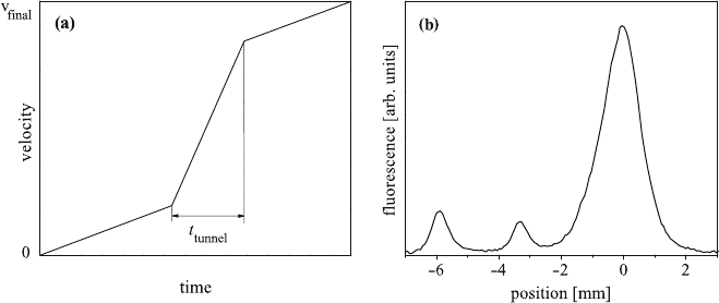
A diagram of the velocity proﬁle versus time is shown in Fig. 8.11(a).

Fig. 8.11 Part (a) shows a diagram of the acceleration sequence to study tunneling out of the

lowest band. Part (b) shows a typical integrated spatial distribution of atoms after ballistic expan-

sion. The large peak on the right is the part of the atomic cloud that was not trapped during the

initial acceleration. The center peak indicates the atoms that tunneled out of the potential during

the fast acceleration period. The leftmost peak corresponds to atoms that remained trapped during

In the detection phase we determined the number of atoms that were initially

trapped and what fraction remained in the ﬁrst band after the tunneling sequence.

After an atom tunneled out of the potential during the sequence, it would maintain

the velocity that it had at the moment of tunneling. During the period of free bal-

listic expansion the difference in ﬁnal velocity between trapped and tunneled atoms

led to their spatial separation (Fig. 8.11(b)). To observe the temporal evolution of

the fundamental band population, we repeated a sequence such as in Fig. 8.11(a)

for various tunneling durations t

tunnel

, holding the other parameters of the sequence

ﬁxed.

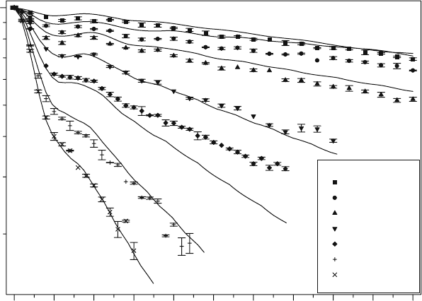
Figure 8.12 shows the probability of survival in the accelerated potential as a

function of the duration of tunneling for various values of the tunneling acceleration

tunnel

between 6000 and 20,000 m/s

. The value for the well depth for all curves

was V

/h = 92 kHz. Initially, the survival probability shows a ﬂat region, owing

to the reversibility of the decay process for short times. At intermediate times the

decay shows a damped oscillation that for long times evolves into the characteris-

tic exponential decay law. By this time the coupling is essentially irreversible and

reformation of the undecayed state is prohibited. As a comparison we also show the

results of quantum mechanical simulations of the entire experimental sequence as

solid lines in the same graph. The tunneling rates depend strongly on the well depth

8 Experiments on Quantum Transport of Ultra-Cold Atoms in Optical Potentials 231

0 5 10 15 20 25 30 35 40 45 50

0.2

0.3

0.4

0.5

0.6

0.7

0.8

0.9

a =6,000m/s

a = 20,000 m/s

a = 17,000 m/s

a = 15,000 m/s

a = 12,000 m/s

a = 10,000 m/s

a =8,000m/s

survival probability

tunneling time [µs]

Fig. 8.12 Probability of survival in the accelerated potential as a function of duration of the tun-

neling acceleration. Data points for different values of the large acceleration a

tunnel

are shown. Each

point represents the average of ﬁve experimental runs, and the error bar denotes the error of the

mean. These data were recorded for a well depth of V

/h = 92 kHz and have been normalized to

unity at t

tunnel

= 0 to compare to the quantum mechanical simulations (shown in solid lines with

no adjustable parameters)

of the potential. Considering the uncertainty of 10% in the calibration of the power

in the interaction beams, the simulations match the observed data quite well.

8.5.4 Quantum Zeno and Anti-Zeno Effects

The universal phenomenon of non-exponential decay of unstable systems led Misra

and Sudarshan in 1977 to the prediction that frequent measurements during this

non-exponential period could inhibit decay entirely [33, 5, 41]. They named this

effect the quantum Zeno effect after the Greek philosopher, famed for his paradoxes

and puzzles. In his most famous paradox, Zeno considers an arrow ﬂying through the

air. The time of ﬂight can be subdivided into inﬁnitesimally small intervals during

which the arrow moves only by inﬁnitesimal amounts. Assuming the summation of

inﬁnitesimal terms amounts to nothing led Zeno to believe that motion is impossi-

ble and is merely an illusion. The version put forth by Misra and Sudarshan is the

quantum mechanical version of the paradox.

To illustrate their main point, we consider the time evolution of a system in

the non-exponential regime, where the probability of remaining in the undecayed

232 M.C. Fischer and M.G. Raizen

state is given by Eq. (8.45). We now subdivide the time t into n time intervals of

length τ and perform a measurement of the system after each interval. Each mea-

surement redeﬁnes a new initial condition and effectively resets the time evolution.

The system must therefore start the evolution again with the same non-exponential

decay features. The probability of remaining in the undecayed state at time t

(after n measurements at intervals τ ) is therefore P(t) =

[

P(τ )

]

, which we can

approximate as

P(t) = exp



−n τ

H







= e

−γ t

, (8.49)

where the decay rate γ is given by

γ = τ

H





. (8.50)

The time evolution of the system that is repeatedly measured is therefore an expo-

nential decay. The remarkable fact is that the decay rate depends on the measure-

ment interval τ and tends to zero as τ goes to zero. Reviews of the quantum Zeno

effect can be found in modern textbooks of quantum mechanics [39]. Even though

measurement-induced suppression of the dynamics of a two-state driven system has

been observed [19, 24], no such effect was ever measured on an unstable system.

Whereas in the previous section we established the non-exponential time depen-

dence, the focus of this section is the effect of measurements on the system decay

rate. The quantity to be measured was the number of atoms remaining trapped in

the potential during the tunneling segment. This measurement could be realized by

suddenly interrupting the tunneling duration by a period of reduced acceleration

interr

, as indicated in Fig. 8.13(a). During this interruption tunneling was negligible

and the atoms were therefore transported to a higher velocity without being lost out

of the well. This separation in velocity space enabled us to distinguish the remaining

atoms from the ones having tunneled out up to the point of interruption, as can be

seen in Fig. 8.13(b). By switching the acceleration back to a

tunnel

, the system was

then returned to its unstable state. The measurement of the number of atoms that

remained trapped deﬁned a new initial state with the remaining number of atoms as

the initial condition. The requirements for this interruption section were very similar

to those during the transport section, namely the largest possible acceleration while

maintaining negligible losses for atoms in the ﬁrst band. Hence a

interr

was chosen to

be the same as a

trans

Figure 8.14 shows the dramatic effect of frequent measurements on the decay

behavior. The hollow squares indicate the decay curve without interruption. The

solid circles in Fig. 8.14 depict the measurement of the survival probability in which

after each tunneling segment of 1 μs an interruption of 50 μs duration was inserted.

Only the short tunneling segments contribute to the total tunneling time. The sur-

vival probability clearly shows a much slower decay than the corresponding system

measured without interruption. Care was taken to include the limited time response

Muga G. Time in Quantum Mechanics - Vol. 2

Подождите немного. Документ загружается.