Muga G. Time in Quantum Mechanics

Подождите немного. Документ загружается.

10 Time Scales and Correlations in Non-Markovian Quantum Open Systems 285

10.4.2 Two-Time Correlation Function of System Observables

in the Non-Markovian Case

Let us take a set of N system observables A

), A

),...,A

) in Heisenberg

representation, such that t

> t

> ··· > t

.IfΨ

is the initial state of the total

system, C

(t) =Ψ

) ···A

)|Ψ

 is an N-time correlation function

of the system. This is the object of our interest.

To begin let us consider the Heisenberg evolution equation for a system observ-

able A(t) = U

−1

(t, 0)AU(t, 0), where U(t, 0) is the evolution operator with the total

Hamiltonian,

dA(t

)

= iU

−1

, 0)[H

, A]U(t

, 0) =−i[H

), A(t

)]



†

, 0)[L(t

), A(t

)] + [L

†

), A(t

)]a

, 0)

. (10.15)

We can replace in (10.15) the formal solution of the evolution equation of the

environmental operators, da

, 0)/dt

= i[H

), a

, 0)] =−iω

, 0) −

L(t

, 0) = e

−iω

a(0, 0) −ig



dτ e

−iω

−τ )

L(τ ) . (10.16)

The single evolution equation (10.15) becomes

dA(t

)

= i[H

), A(t

)] − ν

†

)[L(t

), A(t

)]



dτα

∗

−τ )L

†

(τ )[A(t

), L(t

)] + [L

†

), A(t

)]ν(t

)



dτα(t

−τ )[L

†

), A(t

)]L(τ ) , (10.17)

with α(t) =



−iω

being the environment correlation function. Generally,

for an environment with a large number of degrees of freedoms this function decays

in a typical timescale τ

environment correlation time. We have also deﬁned the

bath operators

†

) =−i



†

(0, 0)e

iω

ν(t

) = i



(0, 0)e

−iω

. (10.18)

From (10.17) the evolution equation of the quantum mean value of A for an initial

state of the form | Ψ

=|ψ

|0, with |0 the vacuum state for the environment,

is equal to

286 D. Alonso and I. de Vega

Ψ

| A(t

) | Ψ

=iΨ

| [H

), A(t

)] | Ψ





dτα(t

−τ )Ψ

| [L

†

), A(t

)]L(τ ) | Ψ





dτα

∗

−τ )Ψ

| L

†

(τ )[A(t

), L(t

)] | Ψ

 .

(10.19)

It is important to note that in dynamical equation (10.17) the environment oper-

ators ν(t) and ν

†

(t) represent an external driving acting on the system due to its

interaction with the environment. These f orces are related to the correlation func-

tion α(t − t



), in fact it can be shown that 0|ν(t)ν

†



)|0=α(t − t



), so that the

environment correlation function is the autocorrelation function of the environment

f orces acting on the system. Furthermore, 0|ν

†

(t)|0=0|ν(t)|0=0.

Let us now calculate the following evolution equation:

dA(t

)B(t

)

= iU

−1

)[H

, A]U(t

)B(t) = i[H

), A(t

)]B(t

)



†

, 0)[L(t

), A(t

)]B(t

)

+[L

†

), A(t

)]a

, 0)B(t

)

(10.20)

The idea again is to eliminate the dependence on the environmental operators once

the average over the total system state is performed. First, we replace the analytical

solution of the creation operator a

†

, 0), so that the term a

†

(0, 0) appears in the left

hand side of the expression and can be eliminated when applying the vacuum initial

state. Second, we move the annihilation operator to the right-hand side by doing the

following:

, 0)B(t

) = U

−1

, t

)BU(t

)

= U

−1

−iω

−t

)

(0, 0)BU(t

) − ig



dτ e

−iω

−τ )

L(τ )B(t

)

= B(t

, 0) −ig



dτ e

−iω

−τ )

L(τ )B(t

) , (10.21)

wherewehaveused

, t

) = e

−iω

−t

)

, t

) − ig



dτ e

−iω

−τ )

L(τ,t

), (10.22)

10 Time Scales and Correlations in Non-Markovian Quantum Open Systems 287

with a

, t

) = a

(0, 0) ≡ a

and [B, a

(0, 0)] = 0. We now insert in the former

expression the solution of a

, 0), which is of the form (10.16), and obtain

, 0)B(t

) = e

−iω

B(t

(0, 0) −ig



dτ e

−iω

−τ )

B(t

)L(τ )

−ig



dτ e

−iω

−τ )

L(τ )B(t

) . (10.23)

Replacing (10.23) by (10.20) and considering the solution of a

†

, 0), we obtain

dA(t

)B(t

)

= i[H

), A(t

)]B(t

) − ν

†

)[L(t

), A(t

)]B(t

)

−



dτα

∗

−τ )L

†

(τ )[L(t

), A(t

)]B(t

) + [L

†

), A(t

)]B(t

)ν(t

)



dτα(t

−τ )[L

†

), A(t

)]L(τ )B(t

)



dτα(t

−τ )[L

†

), A(t

)]B(t

)L(τ ) . (10.24)

The evolution of the quantum mean value A(t

)B(t

) is again obtained by

applying the total initial state on both sides of the former expression. When such

initial state is | ψ

|0, we obtain the following:

dΨ

| A(t

)B(t

) | Ψ



= iΨ

| [H

), A(t

)]B(t

) | Ψ





dτα

∗

−τ )Ψ

| L

†

(τ )[A(t

), L(t

)]B(t

) | Ψ





dτα(t

−τ )Ψ

| [L

†

), A(t

)]L(τ )B(t

) | Ψ





dτα(t

−τ )Ψ

| [L

†

), A(t

)]B(t

)L(τ ) | Ψ

 .

(10.25)

Equations (10.19) and (10.25) represent the evolution of quantum mean values

and two-time correlations, respectively, obtained without the use of any approxima-

tion. However, it is clear that these equations are open, in the sense that quantum

mean values depend on two-time correlations, while two-time correlations depend

on three-time correlations. In general, when no approximations are made, N -time

correlation depends on (N + 1)-time correlations, which gives rise to a hierarchy

structure of MTCF as described in [76].

288 D. Alonso and I. de Vega

At this stage we consider that the system and the environment are weakly cou-

pled. If we deﬁne V

AB = e

−iH

B and A(t) = e

−iH

, we can write

a weak coupling approximations of Eqs. (10.19) and (10.25) up to second order in

the coupling constant (see [34, 75] for details).

Then we obtain the following equation for quantum mean values:

Ψ

| A(t

) | Ψ

=iΨ

{

, A]

}

) | Ψ





dτα

∗

−τ )Ψ



τ −t

†

[A, L]



) | Ψ





dτα(t

−τ )Ψ



†

, A]V

τ −t



) | ψ



(10.26)

and for two-time correlations

Ψ

| A(t

)B(t

) | Ψ

=iΨ

{

, A]

}

)B(t

) | Ψ





dτα

∗

−τ )Ψ



τ −t

†

[A, L]



)B(t

) | Ψ





dτα(t

−τ )Ψ



†

, A]V

τ −t



)B(t

) | ψ





dτα(t

−τ )Ψ



†

, A]



)



[B, V

τ −t



) | Ψ

 .

(10.27)

As noted in [34, 75], while the ﬁrst two terms of (10.27) are analogous to those of

(10.26), the equation for two-time correlations contains an additional term that does

not appear in the evolution of quantum mean values. Note that this term vanishes

for Markovian interactions, since then the correlation α(t

− τ) = Γδ(t

− τ)is0

in the domain of integration from 0 to t

. This result is consistent with the quantum

regression theorem discussed in Sect. 10.4.1.

In conclusion, Eq. (10.27) shall be used in general to evaluate the evolution of

non-Markovian two-time correlations. Moreover, as it is shown in [76], Eqs. (10.26)

and (10.27) are just the ﬁrst two equations of a full hierarchy of equations for multi-

ple time correlations. This hierarchy is closed in the sense that an N-time correlation

function depends at most on other N-time correlations.

Let us remark that it is possible to show that under certain conditions, multiple

time correlation functions evolve as expectation values in the stationary limit, even

in the non-Markovian case [77].

10 Time Scales and Correlations in Non-Markovian Quantum Open Systems 289

In the same vein that for the expectation values, it is possible to compute a par-

ticular multiple time correlation function with a stochastic scheme. We shall discuss

this issue in the next section.

10.4.3 Non-Markovian Stochastic Trajectory Methods for MTCF

It is possible to develop a stochastic scheme to compute multiple time correla-

tion functions. The advantage of this method is that it allows the evaluation of a

speciﬁc correlation function, in contrast to the equations discussed in the previ-

ous sections where the evolution of a certain correlation is coupled to some other

correlations.

If we take the partial interaction picture with respect to the environment, the N-

time correlation function is deﬁned as C

(t|Ψ

)=Ψ

i=1

−1

, 0)A

, 0)|Ψ

,

where U

is the evolution operator of the system in the interaction picture. Within

the Bargmann representation [9, 66], we write

(t|Ψ

) =



dμ(z)ψ

−1

(0, 1)

i=1

G(i, i +1)|ψ

 , (10.28)

with t

= 0, t

N+1

= 0, and z

N+1

= z

. We have introduced the reduced propagators

G(i, i + 1) ≡ G(z

∗

i+1

) =z

, t

i+1

)|z

i+1

, which act on the system

Hilbert space and give the evolution of system state vectors from t

i+1

to t

,given

that in the same time interval the environment coordinates go from z

i+1

to z

.It

is clear then that once their time evolution is solved, the time correlation function

(10.28) can be obtained. It can be shown that the reduced propagator satisﬁes the

evolution equation [34]

∂G(i, i + 1)

∂t



−iH

+ Lz

∗

i,t

− L

†

i+1,t



G(i, i +1)

−L

†



i+1

dτα(t

−τ )z

, t

i+1

)L(τ,t

i+1

)|z

i+1

 ,(10.29)

with L(t



, t) = e

−iH(t−t



)

iH(t−t



)

−iH



.Also,z

i,t

= i



i,n

iω

is a

time-dependent function, α(t − τ ) =



−iω

(t−τ )

, and the initial condition

G(i, i +1) = exp (z

∗

i+1

). Thus the function z

i,t

is a sum of time-dependent coher-

ent states and α(t − τ ) is its time autocorrelation function, as it can be veriﬁed

by computing the average M[z

i,t

∗

i,τ

] regarding the measure dμ(z) as shown in the

previous section:

z

,τ)LU

(τ,t

i+1

) | z

i+1

=M

z

,τ) | z

Lz

| U

(τ,t

i+1

) | z

i+1



= M

G(z

∗

τ )LG(z

∗

i+1

|τ t

i+1

)

, (10.30)

where in the second line we have inserted 1=

−|z|

|zz|, and we have deﬁned

290 D. Alonso and I. de Vega

[···] =



dμ(z

) ··· . (10.31)

With this notation, Eq. (10.29) can be rewritten as

∂G(z

∗

i+1

)

∂t



−iH

+ Lz

∗

i,t

− L

†

i+1,t



G(z

∗

i+1

)

−L

†



i+1

dτα(t

−τ )M

G(z

∗

τ )LG(z

∗

i+1

|τ t

i+1

)

(10.32)

In this equation, the last term expresses how the dissipation at time t depends

on previous trajectories of other system propagators [78]. For that reason, Eq.

(10.29) cannot in general be expressed in terms of the particular propagator evolved

G(i, i + 1), and hence it is not a closed equation for this propagator. Only in very

exceptional cases this can be done in an exact way, while in most of the systems it

is necessary to perform some approximations to close the equation.

One possible approximation is to assume that

z

, t

i+1

)L(τ,t

i+1

)|z

i+1

=O(z

i+1

, t

i+1

,τ)G(i, i + 1) , (10.33)

where the operator O has to be constructed [55], for instance, by treating L(τ,t

i+1

)

in the weak coupling limit. In terms of O(z

i+1

, t

i+1

,τ), Eq. (10.29) reads

∂G(i, i + 1)

∂t



−iH

+ Lz

∗

i,t

− L

†

i+1,t

−L

†



i+1

dτα(t

−τ )O(z

i+1

, t

i+1

,τ)



G(i, i +1) . (10.34)

Equations (10.29) or (10.34) depend on two time-dependent functions, z

∗

i,t

and

i+1,t

, which take into account the “history” of the environment and lead to a con-

ditioned dynamics of the system with respect to the environment dynamics. They

constitute the starting point to compute the non-Markovian MTCFs within a Monte

Carlo method by choosing the variables z

randomly according to the distribution

dμ(z). For a single realization, a value of the integrand appearing in (10.28) can

be obtained; ﬁrst, evolving |ψ

 from (t

N+1

= 0, z

N+1

= z

)to(t

, z

) so that

a vector |φ

=G(N, N + 1)|ψ

, second, applying A

to |φ

 so that we get

=A

|φ

,third,evolving|

 with G(N − 1, N), and so on. The process

continues until the vector |φ

=G(1, 2)|

 is obtained and ﬁnally it is used to

compute ψ

|φ

, with |ψ

=G(0, 1)|ψ

. In the end, the sum over many of

these “histories” with respect to the measure dμ(z) leads to the MTCFs deﬁned in

(10.28).

Notice that since the equation for the reduced propagator (10.29) is made for an

initial state of the environment different from the vacuum, it can be used to compute

10 Time Scales and Correlations in Non-Markovian Quantum Open Systems 291

the expectation values and correlation functions of system observables with more

general initial conditions than the one usually taken, i.e., |Ψ

=|ψ

|0 [64].

The choice between using the stochastic method and the system of equations for

computing the MTCFs has to be made according to the particular problem. When

an N-time correlation function has to be computed with the ﬁrst method, the system

of equations will contain all possible correlations of the matrices Y that form a basis

for the QOS. The correlation of other system observables can be computed by com-

bining correlations of this basic set of observables. In turn, the stochastic method

allows us to compute only the particular correlation function that is needed, and not

the whole set of Y

correlations that appears interrelated in the set of differential

equations. Hence, if the system has a large number of degrees of freedom, so that Y

is a large set, the stochastic method is in general more convenient.

10.5 Examples

To illustrate the theory let us discuss the particular examples of the spontaneous

emission of an atom and the ﬂuorescence in a structured environment.

10.5.1 Atomic Emission Spectra

In this section, we derive the formula necessary to obtain the emission spectra of a

two-level atom in non-Markovian interaction with the surrounding radiation ﬁeld.

We follow a well-known photodetection model of experiment, the gedanken spec-

trum analyzer, that provides an operational deﬁnition of the spectral proﬁle [79].

The Hamiltonian of the emitting atom (with levels |1 and |2)isgivenby

=−

(σ

−σ

) =

, (10.35)

where σ

i, j

=|ij|, with {i, j}=1, 2, are the atomic pseudospin operators in

the atomic basis, and the total Hamiltonian of emitting atom and radiation ﬁeld

is described by a Hamiltonian H

, given by H

= H

+ H



†

L). In order to detect the emitted radiation, suppose that we have a detecting atom

placed in r with Hamiltonian H

= ωσ

/2, where ω is its rotating frequency. The

Hamiltonian of the total system (detector atom, emitting atom, and radiation ﬁeld) is

H = H

+ H

+ W . (10.36)

Here the coupling between the detecting atom H

with H

is dipolar and given by

a Hamiltonian W , which in the interaction picture with respect to the detector is

given by

W(t) =

·E

(+)

(r, t)e

iωt

+σ

·E

(−)

(r, t)e

−iωt

. (10.37)

292 D. Alonso and I. de Vega

Here, we have considered d

= d

=1 | D | 2=d

. The superindex

D reminds that these are the components of the detector’s dipole. It is important to

note here that the ﬁeld operators E

(+)

and E

(−)

correspond to the ﬁeld emitted by

the atoms and the background radiation ﬁeld. The positive part of the ﬁeld at the

position r is deﬁned as

(+)

(r, r

, t) =



(r)a

, t)e

(10.38)

and E

(−)

(r, r

, t) = [E

(+)

(r, r

, t)]

†

[80]. In the last expression (and from now on)

we have added explicitly the dependence on the position r

of the source dipole

(or emitting atom) that originates the ﬁeld. The quantity ε



2ε

, with υ the

quantization volume. In terms of the coupling strengths we ﬁnd that g

≡ g

(r) =

(r)d · e

A shutter is placed between the radiating atom and the detector. In that way,

the radiation illuminates the detector only for the time T in which the shutter is

open. In order to excite the detector, the time of observation T needs to be much

larger than the inverse of the natural width γ of the detecting atom’s excited level.

In addition, T should be larger than the reciprocal of the spectral width 1/Γ of the

emitting atom. With this setup, the spectral distribution of the ﬂuorescence light,

P(ω, T ), is deﬁned as the probability of excitation of the detecting atom at the time

of observation T , i.e.,

P(ω, T ) = Tr

R,D

(

| 22 | ρ(T )

)

, (10.39)

where ρ(T ) is the density matrix of the total system at time T . Replacing the Taylor

expansion of the density matrix ρ(T )forρ(T ) ≈ ρ(0), and after some manipula-

tions, P(ω, T ) is obtained as

P(ω, T ) =





iω(t−t



)

(1)

(r, r

; t, t



) . (10.40)

Here, the average ···=Tr

(

···

)

, and we have deﬁned

(1)

(r, r

; t, t



) =d

·E

(−)

(r, r

, t)d

·E

(+)

(r, r

, t



) (10.41)

as the ﬁrst-order correlation of the projection of the emitted ﬁeld in the direc-

tion of the dipole. In the last expression, the operators d

· E

(−)

(r, r

, t) and

· E

(+)

(r, r

, t



) should be replaced by their expression in terms of the system

operators L

†

and L, respectively. This is done by inserting in (10.38), and in its

complex conjugated, solution (10.16) for a

†

(t, 0) and a



, 0), respectively. Taking

10 Time Scales and Correlations in Non-Markovian Quantum Open Systems 293

into account that the term proportional to a

†

(0, 0) a

(0, 0) does not contribute to

photodetection signals since the ﬁeld is in the vacuum state |0, then

P(ω, T ) =





iω(t−t



)





dτ





dτ



∗

(t −τ )α(t



−τ



)L

†

(τ )L(τ



)



. (10.42)

This formula emphasizes the role of the system ﬂuctuations L

†

(τ )L(τ



) in mea-

surable quantities like the power spectrum of emitted light.

Here it has been assumed that there is no spatial dependence of the environment

correlation function. More details of the derivation can be found in [81].

In the Markov case, the environmental correlation is a delta function, α(t −τ ) =

Γδ(t −τ ), and the last formula is just

P(ω, T ) = Γ





iω(t−t



)

L

†

(t)L(t



) , (10.43)

which in the stationary limit, i.e., with an observation time T →∞, leads to the

usual expression for the power spectra [9]. In addition, within the Markov approx-

imation the system correlations L

†

(0)L(τ ) can be computed with the quantum

regression theorem.

In the non-Markovian case, we cannot assume that the correlation function is a

delta, and it is necessary to use the original formula, (10.42) for the spectra, and the

system of equations (10.27) in order to compute the system correlations.

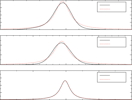
Let us now use formulas (10.42) and (10.43) to compute the non-Markovian

and Markovian spectra, respectively [82], see Fig. 10.1. The non-Markovian case

corresponds to choosing γ small enough so that the correlation function decays

within a nonzero correlation time. Since we are dealing with spontaneous emission

processes, in which the correlation functions L

†

(t)L(t



) relax to a zero value, we

choose the observing time of the detector T > T

, where T

is the relaxation

time of the two-time correlation. Notice that when a laser is tuned to the atomic

rotating frequency, then the two-time correlations do not decay to a zero value, so

that the condition T > T

is not sufﬁcient to obtain a stationary spectrum. In this

case it is necessary to deﬁne the spectra in a stationary limit T →∞.

In the derivation of Eq. (10.42) we have assumed that (10.41) does not depend

on the spatial coordinates and therefore no spatial dependence is considered in the

correlation function of the environment. However, there are systems in which it

is crucial to consider this spatial dependence, for instance, where the evanescent

components of the emitted ﬁeld are relevant [83]. We shall see in the next section an

example in which such spatial dependence has to be taken into account explicitly.

The emission spectra (10.42) are then replaced by a more general expression which

includes the relative position of the detector with respect to the emitting atom:

294 D. Alonso and I. de Vega

Emission Spectrum

−5 0

Γ = 0.4

fitting

−10 −5 0 10

Γ =1

fitting

−100 −50 0 50 100

0.1

0.2

0.3

0.4

Γ = 100

fitting

Fig. 10.1 (Color online) The spontaneous emission spectra are computed with formula (10.42) for

several values of γ , and by choosing T > T

,whereT

is the atomic relaxation time. In order

to observe the departure from the Lorentzian proﬁle typical of Markovian interactions, the result

is numerically ﬁtted with a Lorentzian function. When γ is small, so that non-Markovian effects

are important in the atomic dynamics, the Lorentzian ﬁtting is not appropriate, which means that

the use of formula (10.42) is necessary to compute the spectra. For γ = 100 the interaction is

practically Markovian, and the spectra correspond perfectly to a Lorentzian

P(ω, T ) =





iω(t−t



)

(1)

(r, r

, t, t



)





iω(t−t



)





dτ





dτ



∗

(r, r

, t,τ)S(r, r

, t



,τ



)

×L

†

(τ )L(τ



)



, (10.44)

where

S(r, r

, t,τ) =



−iω

(t−τ )

i(r−r

(10.45)

is the spatially dependent correlation function. In order to compute the ﬂuorescence

spectra, the limit of T →∞has to be taken, so that the signal is observed in the

stationary limit. In that case, the above formula corresponds to a double Laplace

transform of a convolution,

P(ω) = S

∗

(r, r

, −ω)S(r, r

,ω)L

†

(−ω)L(ω) . (10.46)

Muga G. Time in Quantum Mechanics - Vol. 2

Подождите немного. Документ загружается.