Munson B.R. Fundamentals of Fluid Mechanics

Подождите немного. Документ загружается.

where It can also be shown that the displacement and momentum thicknesses are

given by

(9.16)

and

(9.17)

As postulated, the boundary layer is thin provided that is large as Re

S 2.1i.e., d



x S 0Re

™



0.664

1Re



1.721

1Re

 Ux





1Re

9.2 Boundary Layer Characteristics 477

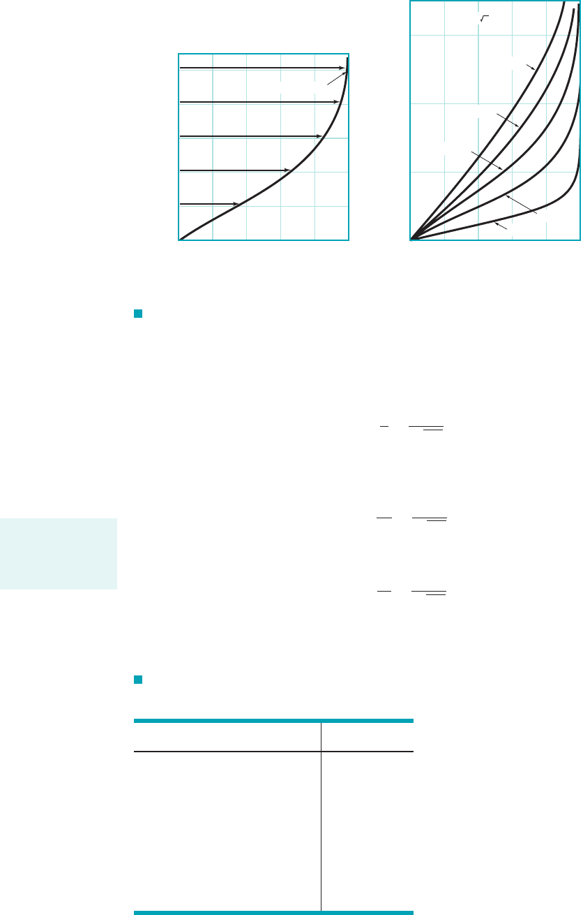
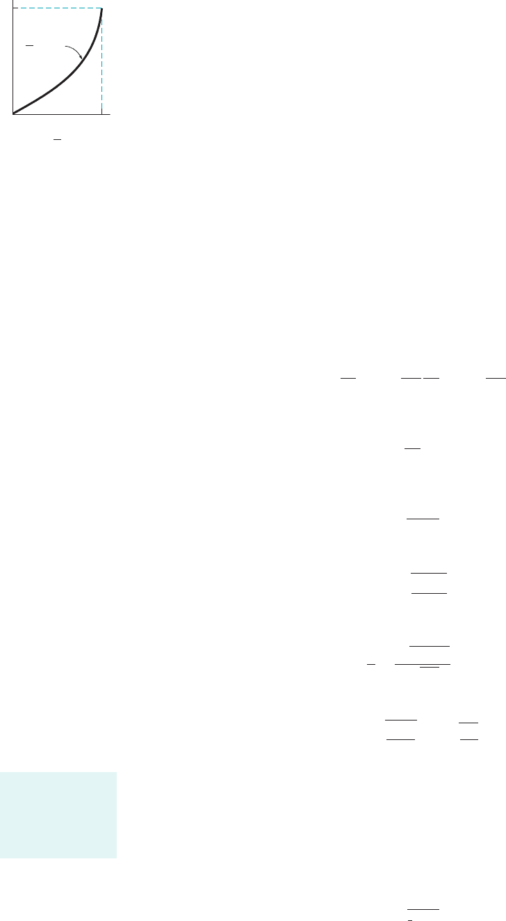
F I G U R E 9.10 Blasius boundary layer profile: (a) boundary layer profile in

dimensionless form using the similarity variable (b) similar boundary layer profiles at

different locations along the flat plate.

= 16 x

= 9 x

= 4 x

x = x

= 25 x

δ ∼

(b)

= 2

= 3

1.00.80.60.40.20

≈ 0.99 at ≈ 5

(a)

′ ( ) =

= y

(

)

TABLE 9.1

Laminar Flow along a Flat Plate

(the Blasius Solution)

( ) () ()

0 0 3.6 0.9233

0.4 0.1328 4.0 0.9555

0.8 0.2647 4.4 0.9759

1.2 0.3938 4.8 0.9878

1.6 0.5168 5.0 0.9916

2.0 0.6298 5.2 0.9943

2.4 0.7290 5.6 0.9975

2.8 0.8115 6.0 0.9990

3.2 0.8761 1.0000

HfⴕHⴝ u



UHfⴕ

1兾2



NxH ⴝ y

For large Reynolds

numbers the bound-

ary layer is rela-

tively thin.

JWCL068_ch09_461-533.qxd 9/23/08 11:47 AM Page 477

With the velocity profile known, it is an easy matter to determine the wall shear stress,

where the velocity gradient is evaluated at the plate. The value of at

can be obtained from the Blasius solution to give

(9.18)

As indicated by Eq. 9.18 and illustrated in the figure in the margin, the shear stress decreases with

increasing x because of the increasing thickness of the boundary layer—the velocity gradient at

the wall decreases with increasing x. Also, varies as not as U as it does for fully devel-

oped laminar pipe flow. These variations are discussed in Section 9.2.3.

9.2.3 Momentum Integral Boundary Layer Equation for a Flat Plate

One of the important aspects of boundary layer theory is the determination of the drag caused by

shear forces on a body. As was discussed in the previous section, such results can be obtained from

the governing differential equations for laminar boundary layer flow. Since these solutions are ex-

tremely difficult to obtain, it is of interest to have an alternative approximate method. The momen-

tum integral method described in this section provides such an alternative.

We consider the uniform flow past a flat plate and the fixed control volume as shown in Fig.

9.11. In agreement with advanced theory and experiment, we assume that the pressure is constant

throughout the flow field. The flow entering the control volume at the leading edge of the plate [sec-

tion 112] is uniform, while the velocity of the flow exiting the control volume [section 122] varies

from the upstream velocity at the edge of the boundary layer to zero velocity on the plate.

The fluid adjacent to the plate makes up the lower portion of the control surface. The upper

surface coincides with the streamline just outside the edge of the boundary layer at section 122. It

need not 1in fact, does not2coincide with the edge of the boundary layer except at section 122. If

we apply the x component of the momentum equation 1Eq. 5.222to the steady flow of fluid within

this control volume we obtain

where for a plate of width b

(9.19)

and is the drag that the plate exerts on the fluid. Note that the net force caused by the uniform

pressure distribution does not contribute to this flow. Since the plate is solid and the upper surface

of the control volume is a streamline, there is no flow through these areas. Thus,

(9.20)d ⫽ rU

bh ⫺ rb

冮

⫺d ⫽ r

冮

112

U1⫺U2 dA ⫹ r

冮

122

⫽⫺d ⫽⫺

冮

plate

dA ⫽⫺b

冮

plate

⫽ r

冮

112

uV ⴢ nˆ dA ⫹ r

冮

122

uV ⴢ nˆ dA

Ⲑ

⫽ 0.332U

Ⲑ

y ⫽ 0

Ⲑ

0yt

⫽ m

10u

Ⲑ

0y2

y⫽0

478 Chapter 9 ■ Flow over Immersed Bodies

√

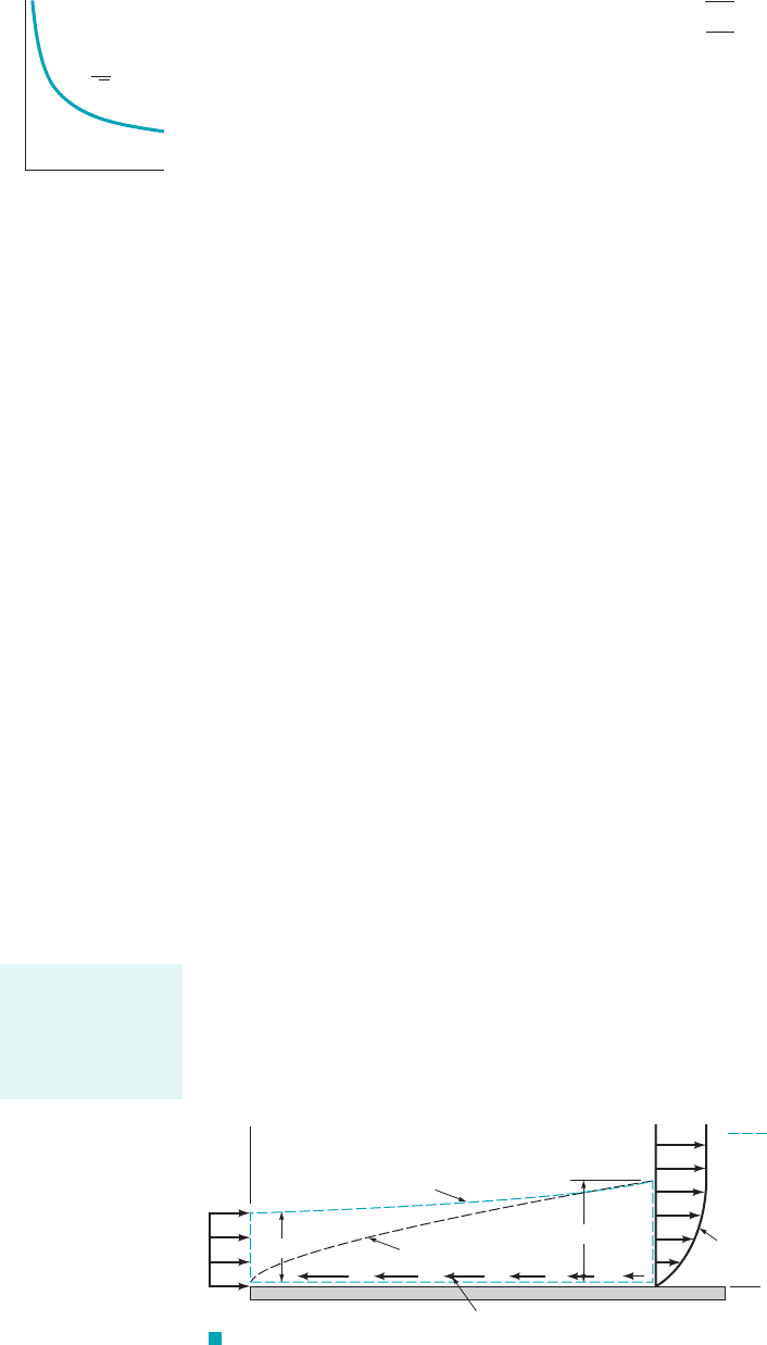
F I G U R E 9.11 Control volume used in the derivation of the

momentum integral equation for boundary layer flow.

Streamline

Boundary layer edge

Control

surface

(2)(1)

(x)

The drag on a flat

plate depends on

the velocity profile

within the bound-

ary layer.

JWCL068_ch09_461-533.qxd 9/23/08 11:47 AM Page 478

Although the height h is not known, it is known that for conservation of mass the flowrate

through section 112must equal that through section 122, or

which can be written as

(9.21)

Thus, by combining Eqs. 9.20 and 9.21 we obtain the drag in terms of the deficit of momentum

flux across the outlet of the control volume as

(9.22)

The idea of a momentum deficit is illustrated in the figure in the margin. If the flow

were inviscid, the drag would be zero, since we would have and the right-hand side of

Eq. 9.22 would be zero. 1This is consistent with the fact that if .2Equation 9.22

points out the important fact that boundary layer flow on a flat plate is governed by a balance

between shear drag 1the left-hand side of Eq. 9.222and a decrease in the momentum of the

fluid 1the right-hand side of Eq. 9.222. As x increases, increases and the drag increases. The

thickening of the boundary layer is necessary to overcome the drag of the viscous shear stress

on the plate. This is contrary to horizontal fully developed pipe flow in which the momentum

of the fluid remains constant and the shear force is overcome by the pressure gradient along

the pipe.

The development of Eq. 9.22 and its use was first put forth in 1921 by T. von

Kármán 11881–19632, a Hungarian/German aerodynamicist. By comparing Eqs. 9.22 and 9.4 we

see that the drag can be written in terms of the momentum thickness, as

(9.23)

Note that this equation is valid for laminar or turbulent flows.

The shear stress distribution can be obtained from Eq. 9.23 by differentiating both sides with

respect to x to obtain

(9.24)

The increase in drag per length of the plate, occurs at the expense of an increase of the

momentum boundary layer thickness, which represents a decrease in the momentum of the fluid.

Since 1see Eq. 9.192it follows that

(9.25)

Hence, by combining Eqs. 9.24 and 9.25 we obtain the momentum integral equation for the bound-

ary layer flow on a flat plate

(9.26)

The usefulness of this relationship lies in the ability to obtain approximate boundary layer

results easily by using rather crude assumptions. For example, if we knew the detailed velocity

profile in the boundary layer 1i.e., the Blasius solution discussed in the previous section2, we could

evaluate either the right-hand side of Eq. 9.23 to obtain the drag, or the right-hand side of Eq. 9.26

to obtain the shear stress. Fortunately, even a rather crude guess at the velocity profile will allow

us to obtain reasonable drag and shear stress results from Eq. 9.26. This method is illustrated in

Example 9.4.

⫽ rU

d™

⫽ bt

dd ⫽ t

b dx

Ⲑ

dx,

⫽ rbU

d™

d ⫽ rbU

™

™,

m ⫽ 0t

⫽ 0

u K U

d ⫽ rb

冮

u1U ⫺ u2 dy

bh ⫽ rb

冮

Uu dy

Uh ⫽

冮

u dy

9.2 Boundary Layer Characteristics 479

Drag on a flat plate

is related to mo-

mentum deficit

within the bound-

ary layer.

U – u

(U – u)

JWCL068_ch09_461-533.qxd 9/23/08 11:47 AM Page 479

As is illustrated in Example 9.4, the momentum integral equation, Eq. 9.26, can be used

along with an assumed velocity profile to obtain reasonable, approximate boundary layer results.

The accuracy of these results depends on how closely the shape of the assumed velocity profile

approximates the actual profile.

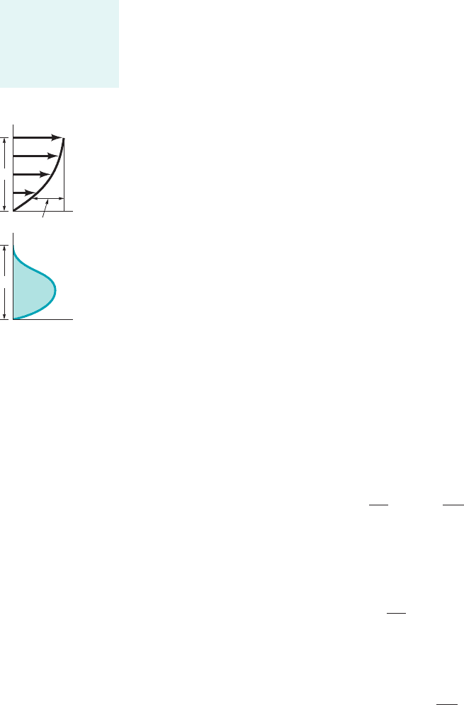
Thus, we consider a general velocity profile

and

where the dimensionless coordinate varies from 0 to 1 across the boundary layer. The

dimensionless function can be any shape we choose, although it should be a reasonableg1Y2

Y  y



 1

for

Y 7 1

 g1Y2

for

0  Y  1

480 Chapter 9 ■ Flow over Immersed Bodies

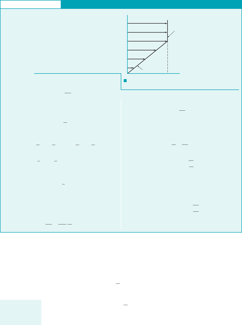
GIVEN Consider the laminar flow of an incompressible fluid

past a flat plate at The boundary layer velocity profile is

approximated as for and for

as is shown in Fig. E9.4.

FIND Determine the shear stress by using the momentum inte-

gral equation. Compare these results with the Blasius results

given by Eq. 9.18.

y 7 d,u  U0  y  du  Uy



y  0.

OLUTION

F I G U R E E9.4

Momentum Integral Boundary Layer Equation

This can be integrated from the leading edge of the plate,

1where 2to an arbitrary location x where the boundary layer

thickness is The result is

(4)

Note that this approximate result 1i.e., the velocity profile is not ac-

tually the simple straight line we assumed2compares favorably with

the 1much more laborious to obtain2Blasius result given by Eq. 9.15.

The wall shear stress can also be obtained by combining Eqs.

1, 3, and 4 to give

(Ans)

Again this approximate result is close 1within 13%2to the

Blasius value of given by Eq. 9.18.t

 0.289U



d  3.46



d  0

x  0

d dd 

u = Uy/

u = U

XAMPLE 9.4

From Eq. 9.26 the shear stress is given by

(1)

while for laminar flow we know that For the

assumed profile we have

(2)

and from Eq. 9.4

(3)

Note that as yet we do not know the value of 1but suspect that it

should be a function of x2.

By combining Eqs. 1, 2, and 3 we obtain the following differ-

ential equation for



™ 



冮

b a1 

b dy

™ 

冮

a1 

b dy 

冮

a1 

b dy

 m

 m10u



0y2

y0

 rU

d™

Approximate veloc-

ity profiles are used

in the momentum

integral equation.

JWCL068_ch09_461-533.qxd 9/23/08 11:47 AM Page 480

approximation to the boundary layer profile, as shown by the figure in the margin. In partic-

ular, it should certainly satisfy the boundary conditions at and at

That is,

The linear function used in Example 9.4 is one such possible profile. Other conditions,

such as at could also be incorporated into the func-

tion to more closely approximate the actual profile.

For a given the drag can be determined from Eq. 9.22 as

(9.27)

where the dimensionless constant has the value

Also, the wall shear stress can be written as

(9.28)

where the dimensionless constant has the value

By combining Eqs. 9.25, 9.27, and 9.28 we obtain

which can be integrated from at to give

(9.29)

By substituting this expression back into Eqs. 9.28 we obtain

(9.30)

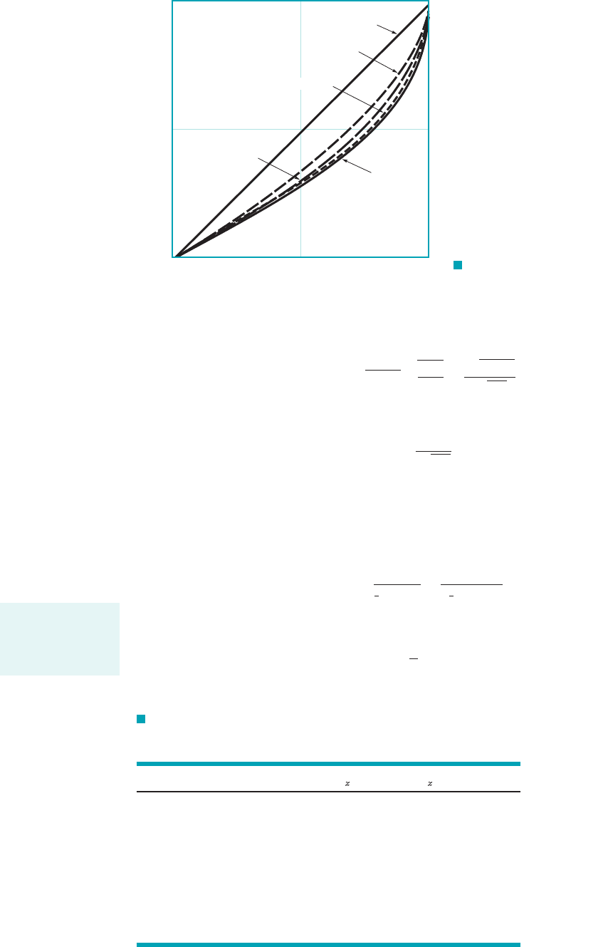
To use Eqs. 9.29 and 9.30 we must determine the values of and Several assumed ve-

locity profiles and the resulting values of are given in Fig. 9.12 and Table 9.2. The more closely

the assumed shape approximates the actual 1i.e., Blasius2profile, the more accurate the final re-

sults. For any assumed profile shape, the functional dependence of and on the physical para-

meters and x is the same. Only the constants are different. That is, or

and where

It is often convenient to use the dimensionless local friction coefficient, defined as

(9.31)c

⫽

⫽ rUx

Ⲑ

m.t

⬃ 1rmU

Ⲑ

,dRe

Ⲑ

x ⫽ constant,

d ⬃ 1mx

Ⲑ

rU2

Ⲑ

r, m, U,

⫽

Ⲑ

⫽

12C

Ⲑ

1Re

d ⫽

2nC

x ⫽ 0d ⫽ 0

d dd ⫽

rUC

⫽

Y⫽0

⫽ m

y⫽0

⫽

Y⫽0

⫽

冮

g1Y231 ⫺ g1Y24 dY

d ⫽ rbU

d ⫽ rb

冮

u1U ⫺ u2 dy ⫽ rbU

冮

g1Y231 ⫺ g1Y24 dY

g1Y2,

g1Y2

1i.e., 0u

Ⲑ

0y ⫽ 0 at y ⫽ d2,Y ⫽ 1dg

Ⲑ

dY ⫽ 0

g1Y2⫽ Y

g102⫽ 0

and

g112⫽ 1

y ⫽ d.u ⫽ Uy ⫽ 0u ⫽ 0

9.2 Boundary Layer Characteristics 481

g(Y)

Approximate

boundary layer re-

sults are obtained

from the momentum

integral equation.

JWCL068_ch09_461-533.qxd 9/23/08 11:47 AM Page 481

to express the wall shear stress. From Eq. 9.30 we obtain the approximate value

while the Blasius solution result is given by

(9.32)

These results are also indicated in Table 9.2.

For a flat plate of length and width b, the net friction drag, can be expressed in terms

of the friction drag coefficient, as

(9.33)C

⫽

冮

⫽

冮

⫽

0.664

1Re

⫽ 12C

rUx

⫽

12C

1Re

482 Chapter 9 ■ Flow over Immersed Bodies

Parabolic

Blasius

Sine wave

Cubic

Linear

1.00.50

0.5

1.0

F I G U R E 9.12 Typical

approximate boundary layer profiles

used in the momentum integral equation.

TABLE 9.2

Flat Plate Momentum Integral Results for Various Assumed

Laminar Flow Velocity Profiles

Profile Character

a. Blasius solution 5.00 0.664 1.328

b. Linear

3.46 0.578 1.156

c. Parabolic

5.48 0.730 1.460

d. Cubic

4.64 0.646 1.292

e. Sine wave

4.79 0.655 1.310u

Ⲑ

U ⫽ sin3p1y

Ⲑ

U ⫽ 31y

Ⲑ

2 ⫺ 1y

Ⲑ

U ⫽ 2y

Ⲑ

d ⫺ 1y

Ⲑ

U ⫽ y

Ⲑ

ᐍ

Ⲑ

DRe

Ⲑ

The friction drag

coefficient is an in-

tegral of the local

friction coefficient.

JWCL068_ch09_461-533.qxd 9/23/08 11:47 AM Page 482

We use the above approximate value of to obtain

where is the Reynolds number based on the plate length. The corresponding value ob-

tained from the Blasius solution 1Eq. 9.322and shown by the figure in the margin gives

These results are also indicated in Table 9.2.

The momentum integral boundary layer method provides a relatively simple technique to ob-

tain useful boundary layer results. As is discussed in Sections 9.2.5 and 9.2.6, this technique can

be extended to boundary layer flows on curved surfaces 1where the pressure and fluid velocity at

the edge of the boundary layer are not constant2and to turbulent flows.

9.2.4 Transition from Laminar to Turbulent Flow

The analytical results given in Table 9.2 are restricted to laminar boundary layer flows along a flat

plate with zero pressure gradient. They agree quite well with experimental results up to the point

where the boundary layer flow becomes turbulent, which will occur for any free-stream velocity

and any fluid provided the plate is long enough. This is true because the parameter that governs

the transition to turbulent flow is the Reynolds number—in this case the Reynolds number based

on the distance from the leading edge of the plate,

The value of the Reynolds number at the transition location is a rather complex function of

various parameters involved, including the roughness of the surface, the curvature of the surface 1for

example, a flat plate or a sphere2, and some measure of the disturbances in the flow outside the

boundary layer. On a flat plate with a sharp leading edge in a typical airstream, the transition takes

place at a distance x from the leading edge given by to Unless otherwise

stated, we will use in our calculations.

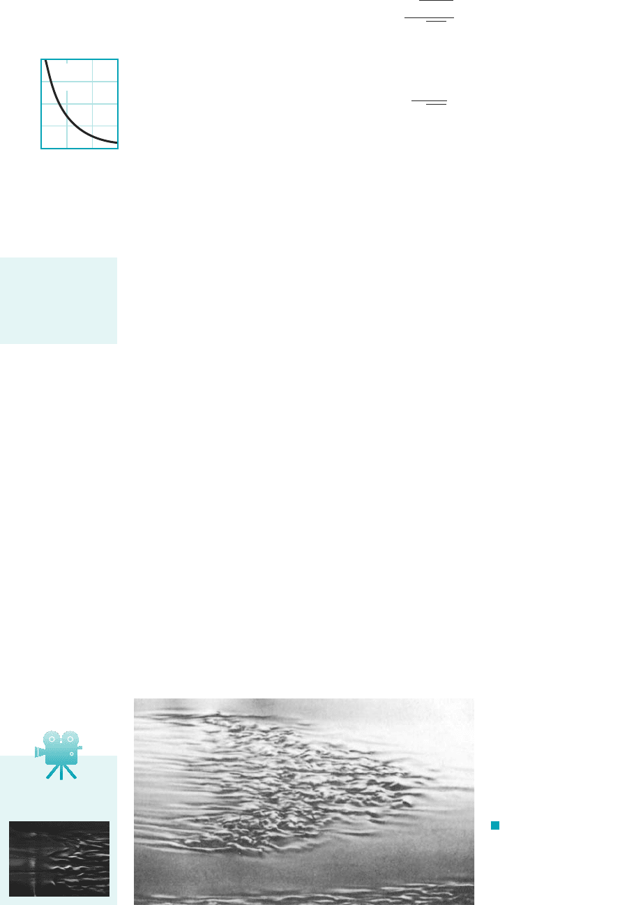
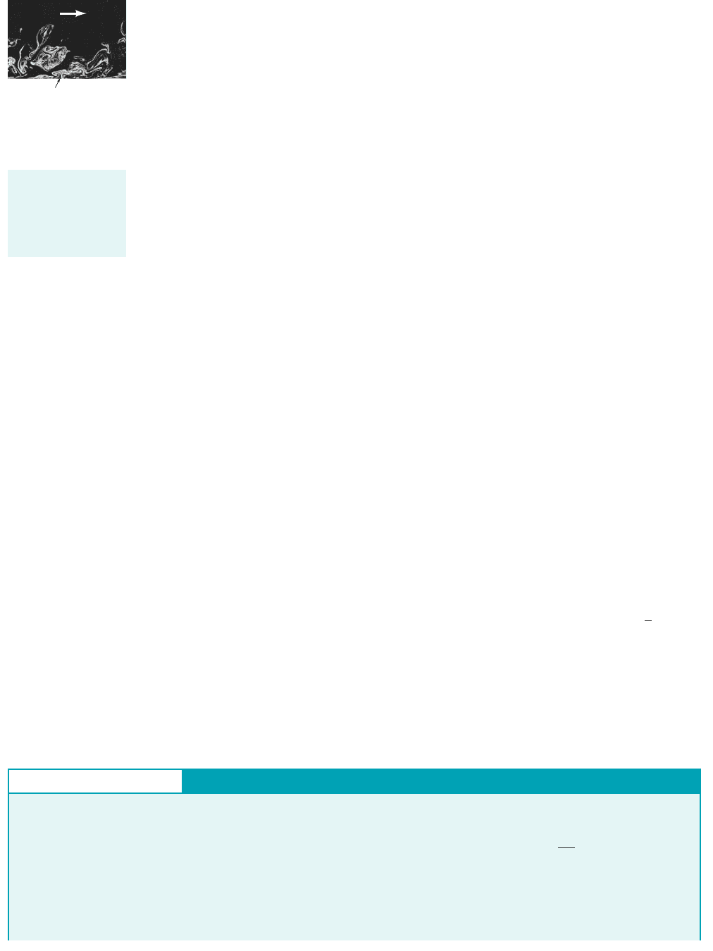
The actual transition from laminar to turbulent boundary layer flow may occur over a region

of the plate, not at a specific single location. This occurs, in part, because of the spottiness of the

transition. Typically, the transition begins at random locations on the plate in the vicinity of

These spots grow rapidly as they are convected downstream until the entire width of the

plate is covered with turbulent flow. The photo shown in Fig. 9.13 illustrates this transition process.

The complex process of transition from laminar to turbulent flow involves the instability of the

flow field. Small disturbances imposed on the boundary layer flow 1i.e., from a vibration of the plate,

a roughness of the surface, or a “wiggle” in the flow past the plate2will either grow 1instability2or

decay 1stability2, depending on where the disturbance is introduced into the flow. If these disturbances

occur at a location with they will die out, and the boundary layer will return to laminar

flow at that location. Disturbances imposed at a location with will grow and transform

the boundary layer flow downstream of this location into turbulence. The study of the initiation,

growth, and structure of these turbulent bursts or spots is an active area of fluid mechanics research.

7 Re

xcr

6 Re

xcr

⫽ Re

xcr

⫽ 5 ⫻ 10

3 ⫻ 10

.Re

xcr

⫽ 2 ⫻ 10

⫽ Ux

Ⲑ

⫽

1.328

1Re

⫽ U/

Ⲑ

⫽

18C

1Re

⫽ 12C

Ⲑ

rUx2

Ⲑ

9.2 Boundary Layer Characteristics 483

0.04

0.03

Laminar

boundary

layer

0.02

0.01

0.00

ᐉ

F I G U R E 9.13

Turbulent spots and the tran-

sition from laminar to turbulent

boundary layer flow on a flat

plate. Flow from left to right.

(Photograph courtesy of

B. Cantwell, Stanford University.)

V9.5 Transition on

flat plate

The boundary layer

on a flat plate will

become turbulent if

the plate is long

enough.

JWCL068_ch09_461-533.qxd 9/23/08 11:47 AM Page 483

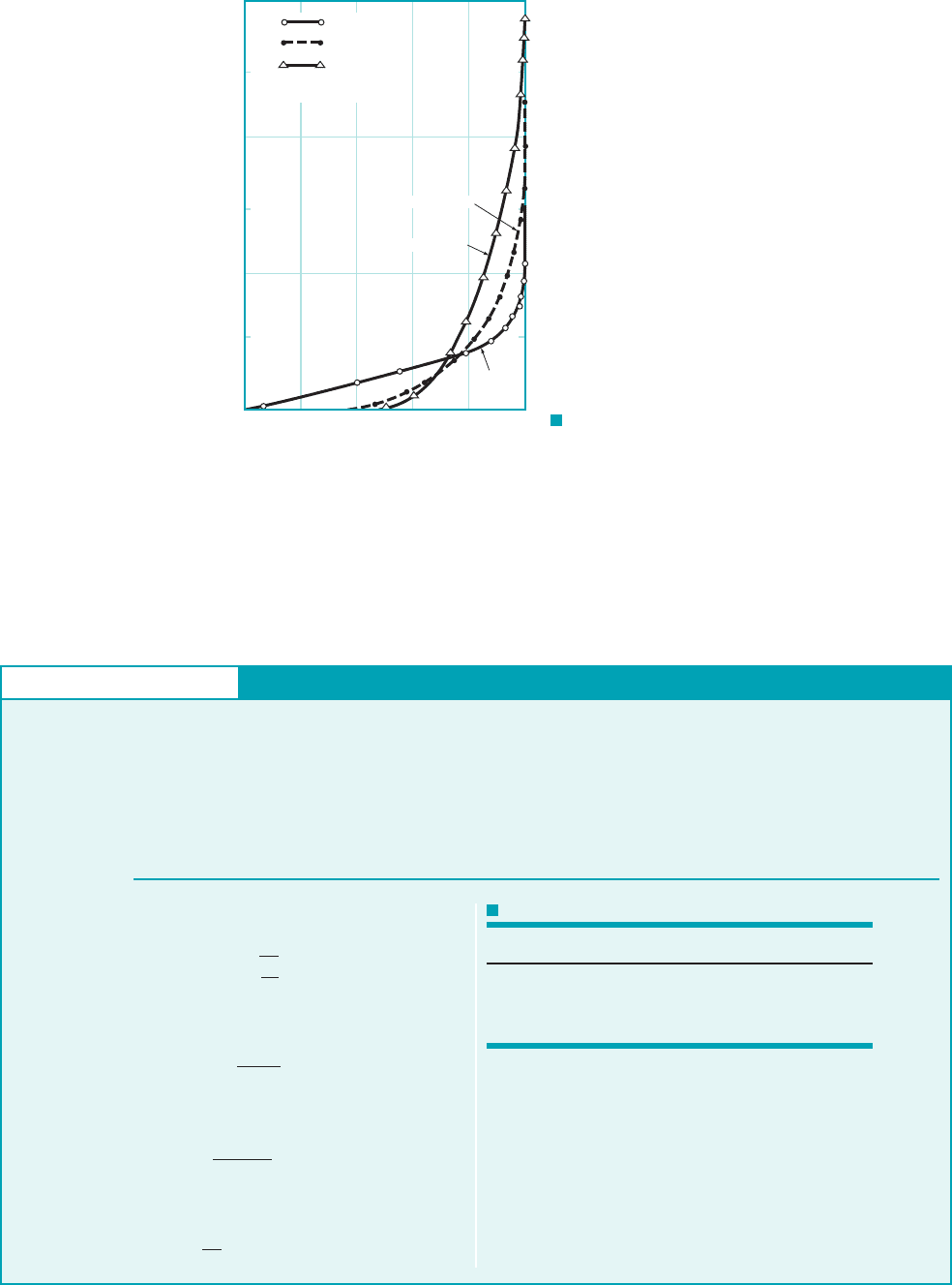
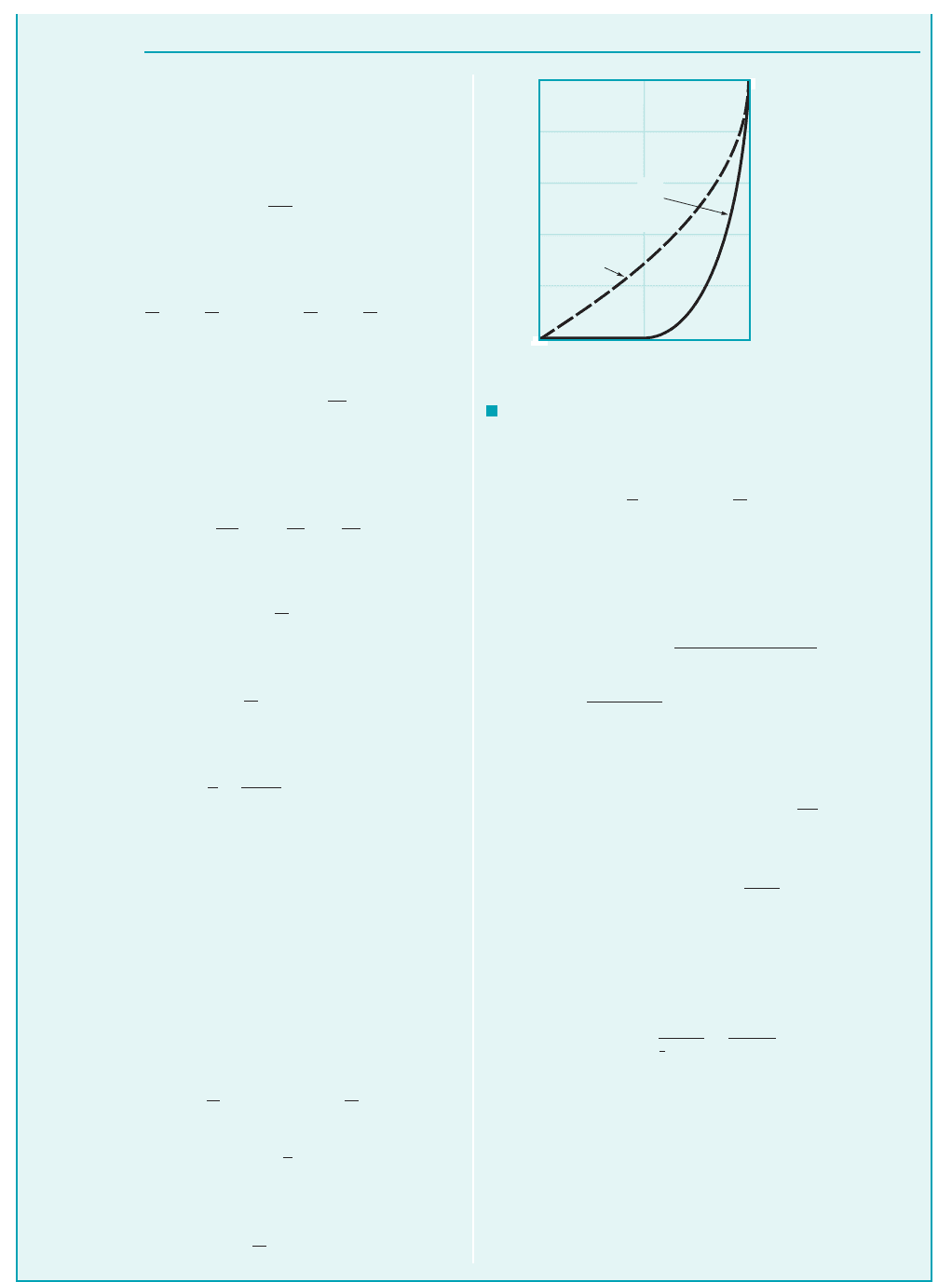
Transition from laminar to turbulent flow also involves a noticeable change in the shape of

the boundary layer velocity profile. Typical profiles obtained in the neighborhood of the transition

location are indicated in Fig. 9.14. The turbulent profiles are flatter, have a larger velocity gradi-

ent at the wall, and produce a larger boundary layer thickness than do the laminar profiles.

484 Chapter 9 ■ Flow over Immersed Bodies

F I G U R E 9.14 Typical boundary layer

profiles on a flat plate for laminar, transitional, and turbu-

lent flow (Ref. 1).

x = 5.25 ft

x = 6.76 ft

x = 8.00 ft

U = 89 ft/s; air flow

Transitional

Turbulent

Laminar

0.06

0.05

0.04

0.03

0.02

0.01

y, ft

0 0.2 0.4 0.6 0.8 1

GIVEN A fluid flows steadily past a flat plate with a velocity

FIND At approximately what location will the boundary layer

become turbulent, and how thick is the boundary layer at that

U ⫽ 10 ft

Ⲑ

point if the fluid is 1a2water at 1b2standard air, or

1c2glycerin at 68 °F?

60 °F,

OLUTION

Boundary Layer Transition

where is in and and are in feet. The values of the

kinematic viscosity obtained from Tables 1.5 and 1.7 are listed in

Table E9.5 along with the corresponding and

COMMENT Laminar flow can be maintained on a longer

portion of the plate if the viscosity is increased. However, the

boundary layer flow eventually becomes turbulent, provided the

plate is long enough. Similarly, the boundary layer thickness is

greater if the viscosity is increased.

Ⲑ

XAMPLE 9.5

For any fluid, the laminar boundary layer thickness is found from

Eq. 9.15 as

The boundary layer remains laminar up to

Thus, if we assume we obtain

and

 d 0

x⫽x

⫽ 5c

15 ⫻ 10

n2d

Ⲑ

⫽ 354 n

⫽

5 ⫻ 10

10 ft

Ⲑ

n ⫽ 5 ⫻ 10

xcr

⫽ 5 ⫻ 10

⫽

nRe

xcr

d ⫽ 5

TABLE E9.5

Fluid ( ) (ft) (ft)

a. Water 0.605 0.00428

b. Air 7.85 0.0556

c. Glycerin 640.0 4.53 1.28 ⫻ 10

⫺2

1.57 ⫻ 10

⫺4

1.21 ⫻ 10

⫺5

Ⲑ

(Ans)

JWCL068_ch09_461-533.qxd 9/23/08 11:47 AM Page 484

9.2.5 Turbulent Boundary Layer Flow

The structure of turbulent boundary layer flow is very complex, random, and irregular. It shares

many of the characteristics described for turbulent pipe flow in Section 8.3. In particular, the veloc-

ity at any given location in the flow is unsteady in a random fashion. The flow can be thought of as

a jumbled mix of intertwined eddies 1or swirls2of different sizes 1diameters and angular velocities2.

The figure in the margin shows a laser-induced fluorescence visualization of a turbulent boundary

layer on a flat plate (side view). The various fluid quantities involved 1i.e., mass, momentum, en-

ergy2are convected downstream in the free-stream direction as in a laminar boundary layer. For tur-

bulent flow they are also convected across the boundary layer 1in the direction perpendicular to the

plate2by the random transport of finite-sized fluid particles associated with the turbulent eddies.

There is considerable mixing involved with these finite-sized eddies—considerably more than is

associated with the mixing found in laminar flow where it is confined to the molecular scale. Al-

though there is considerable random motion of fluid particles perpendicular to the plate, there is

very little net transfer of mass across the boundary layer—the largest flowrate by far is parallel to

the plate.

There is, however, a considerable net transfer of x component of momentum perpendicular

to the plate because of the random motion of the particles. Fluid particles moving toward the plate

1in the negative y direction2have some of their excess momentum 1they come from areas of higher

velocity2removed by the plate. Conversely, particles moving away from the plate 1in the positive

y direction2gain momentum from the fluid 1they come from areas of lower velocity2. The net re-

sult is that the plate acts as a momentum sink, continually extracting momentum from the fluid.

For laminar flows, such cross-stream transfer of these properties takes place solely on the mole-

cular scale. For turbulent flow the randomness is associated with fluid particle mixing. Conse-

quently, the shear force for turbulent boundary layer flow is considerably greater than it is for

laminar boundary layer flow 1see Section 8.3.22.

There are no “exact” solutions for turbulent boundary layer flow. As is discussed in Section

9.2.2, it is possible to solve the Prandtl boundary layer equations for laminar flow past a flat plate

to obtain the Blasius solution 1which is “exact” within the framework of the assumptions involved

in the boundary layer equations2. Since there is no precise expression for the shear stress in turbu-

lent flow 1see Section 8.32, solutions are not available for turbulent flow. However, considerable

headway has been made in obtaining numerical 1computer2solutions for turbulent flow by using

approximate shear stress relationships. Also, progress is being made in the area of direct, full nu-

merical integration of the basic governing equations, the Navier–Stokes equations.

Approximate turbulent boundary layer results can also be obtained by use of the momen-

tum integral equation, Eq. 9.26, which is valid for either laminar or turbulent flow. What is

needed for the use of this equation are reasonable approximations to the velocity profile

where and u is the time-averaged velocity 1the overbar notation, of Sec-

tion 8.3.2 has been dropped for convenience2, and a functional relationship describing the wall

shear stress. For laminar flow the wall shear stress was used as In theory,

such a technique should work for turbulent boundary layers also. However, as is discussed in

Section 8.3, the details of the velocity gradient at the wall are not well understood for turbulent

flow. Thus, it is necessary to use some empirical relationship for the wall shear stress. This is

illustrated in Example 9.6.

 m10u



0y2

y0

u,Y  y



du  U g1Y2,

9.2 Boundary Layer Characteristics 485

Random transport

of finite-sized fluid

particles occurs

within turbulent

boundary layers.

Plate

GIVEN Consider turbulent flow of an incompressible fluid

past a flat plate. The boundary layer velocity profile is assumed

to be for and for

as shown in Fig. E9.6. This is a reasonable approxima-

tion of experimentally observed profiles, except very near the

plate where this formula gives at Note the

differences between the assumed turbulent profile and the lami-

nar profile. Also assume that the shear stress agrees with the

y  0.0u



0y  q

Y 7 1

u  UY  y



d  1u



U  1y



 Y



experimentally determined formula:

(1)

FIND Determine the boundary layer thicknesses and

and the wall shear stress, as a function of x. Determine the

friction drag coefficient, C

™d, d*,

 0.0225rU



Turbulent Boundary Layer Properties

XAMPLE 9.6

JWCL068_ch09_461-533.qxd 9/23/08 11:47 AM Page 485

486 Chapter 9 ■ Flow over Immersed Bodies

OLUTION

Similarly, from Eq. 2,

(4) (Ans)

The functional dependence for and is the same; only the

constants of proportionality are different. Typically,

By combining Eqs. 1 and 3, we obtain the following result for

the wall shear stress

(Ans)

This can be integrated over the length of the plate to obtain the

friction drag on one side of the plate, as

where is the area of the plate. 1This result can also be ob-

tained by combining Eq. 9.23 and the expression for the momen-

tum thickness given in Eq. 4.2The corresponding friction drag

coefficient, is

(Ans)

COMMENT Note that for the turbulent boundary layer flow

the boundary layer thickness increases with x as and the

shear stress decreases as For laminar flow these de-

pendencies are and respectively. The random charac-

ter of the turbulent flow causes a different structure of the flow.

Obviously the results presented in this example are valid only

in the range of validity of the original data—the assumed veloc-

ity profile and shear stress. This range covers smooth flat plates

with 5 ⫻ 10

6 Re

6 10

⫺1

Ⲑ

⬃ x

⫺1

Ⲑ

d ⬃ x

Ⲑ

⫽

0.0720

Ⲑ

A ⫽ b/

⫽ 0.0360rU

Ⲑ

⫽

冮

dx ⫽ b10.0288rU

冮

Ⲑ

⫽

0.0288rU

Ⲑ

⫽ 0.0225rU

U10.37021n

Ⲑ

™6d* 6 d.

™d, d*,

™ ⫽

d ⫽ 0.0360 a

Ⲑ

Whether the flow is laminar or turbulent, it is true that the drag

force is accounted for by a reduction in the momentum of the

fluid flowing past the plate. The shear is obtained from Eq. 9.26

in terms of the rate at which the momentum boundary layer thick-

ness, increases with distance along the plate as

For the assumed velocity profile, the boundary layer momen-

tum thickness is obtained from Eq. 9.4 as

or by integration

(2)

where is an unknown function of x. By combining the assumed

shear force dependence 1Eq. 12with Eq. 2, we obtain the follow-

ing differential equation for

This can be integrated from at to obtain

(3)

(Ans)

or in dimensionless form

Strictly speaking, the boundary layer near the leading edge of

the plate is laminar, not turbulent, and the precise boundary

condition should be the matching of the initial turbulent bound-

ary layer thickness 1at the transition location2with the thickness

of the laminar boundary layer at that point. In practice, how-

ever, the laminar boundary layer often exists over a relatively

short portion of the plate, and the error associated with starting

the turbulent boundary layer with at can be negli-

gible.

The displacement thickness, and the momentum thickness,

can be obtained from Eqs. 9.3 and 9.4 by integrating as fol-

lows:

Thus, by combining this with Eq. 3 we obtain

(Ans)

d* ⫽ 0.0463 a

Ⲑ

⫽ d

冮

11 ⫺ Y

Ⲑ

2 dY ⫽

d* ⫽

冮

a1 ⫺

b dy ⫽ d

冮

a1 ⫺

b dY

™,

d*,

x ⫽ 0d ⫽ 0

⫽

0.370

Ⲑ

d ⫽ 0.370 a

Ⲑ

x ⫽ 0d ⫽ 0

Ⲑ

dd ⫽ 0.231 a

Ⲑ

0.0225rU

Ⲑ

⫽

™ ⫽ d

冮

Ⲑ

11 ⫺ Y

Ⲑ

2 dY ⫽

™ ⫽

冮

a1 ⫺

b dy ⫽ d

冮

a1 ⫺

b dY

⫽ rU

d™

™,

F I G U R E E9.6

Laminar

Turbulent

1.00.50

0.2

0.4

0.6

0.8

1.0

Y =

(

)

JWCL068_ch09_461-533.qxd 9/23/08 11:47 AM Page 486