Odekon M. Encyclopedia of paleoclimatology and ancient environments

Подождите немного. Документ загружается.

bifurcations (Figure Q1e). This means the forcing required to

cause a climate transition is different from that needed to

reverse it. This bifurcation of the climate system has been

inferred from ocean models which mimic the impact of fresh-

water (control variable) on deep-water formation in the North

Atlantic (climate variable) (e.g., Rahmstorf, 1995). However,

a bifurcation relationship could be applied to many forcing

mechanisms and the corresponding responses of the global

climate system. For example, Maslin (2004b) applied it to rain-

fall control on rainforest versus savannah vegetation in the

tropics. Figure Q2 demonstrates this bifurcation of the climate

system and shows that different relationships exist between

climate and forcing mechanism, depending on the direction of

the threshold. This is very common in natural systems, for

example in cases where inertia or the shift between different

states of matter need to be overcome. Figure Q2 shows that

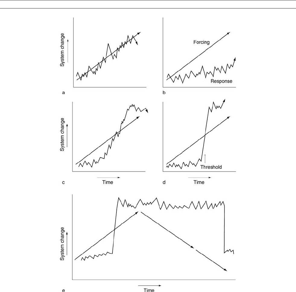
Figure Q1 Schematic diagram of the four alternative responses of the global climate system to internal or external forcing: (a) Linear and

synchronous response: forcing produces a direct response with a magnitude that is proportional to the forcing. (b) Muted or limited response:

forcing may be extremely strong, but the climate system is in some way buffered and therefore has very little response. (c) Delayed or non-linear

response: the climate system may respond slowly to the forcing or is in some way buffered initially, but then responds to the forcing in a non-

linear way. (d) Threshold response: very little or no response to the forcing initially, however all the response then takes place in a very short period

in one large step or threshold. In many cases, the response may be much larger than expected from the size of the forcing, leading to a response

over-shoot. (e) Bifurcation. Similar to the threshold response except that reversing the forcing does not reverse the climate response, see

Figure Q2.

842 QUATERNARY CLIMATE TRANSITIONS AND CYCLES

in cases A and B, the system is reversible, but in case C, it is

not. Figure Q1e shows how case C would manifest itself if

the outcome were plotted on a forcing-response diagram.

In this paper, current theories on major transitions and

cycles within the Quaternary period are reviewed, always con-

sidering the modes of climate changed discussed above. These

include the Intensification of Northern Hemisphere Glaciation

(2.5 Ma), intensification of the Walker Circulation (1.9 Ma),

glacial-interglacial cycles, Mid-Pleistocene Revolution (1Ma),

quasi-periodic millennial climate cycles and the last glacial-

Holocene transition (Figure Q3).

Onset and int ensification of Northern Hemisphere

glaciation

Heralding the start of the Quaternary period

The earliest recorded onset of significant global glaciation during

the last 100 Ma was the widespread continental glaciation of

Antarctica at about 34 Ma (e.g., Zachos et al., 2001). Records

indicate that ice rafting started in the Arctic as early as 46 Ma

(Eldrett et al., 2007) but major glaciation did not occur until

14–6 Ma (Thiede et al., 1998). Marked expansion of continental

ice sheets in the Northern Hemisphere was the culmination of a

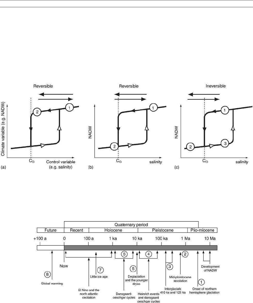
Figure Q2 Bifurcation of the global climate system. For example, the control variable could be North Atlantic salinity and the climate variable

could be production of NADW. (a) An insensitive system in which the climate variable does not vary greatly with large changes in the control

variable. (b) The control variable drops beneath the critical threshold point C

(point 2), causing a major change in the climate variable; however,

by returning the control variable to its original state, the system is reversible and the climate variable returns to its original point 1. (c) The control

variable drops beneath the critical threshold point C

(point 2); however, returning the control variable to its original state does not reverse the

change and the climate variable remains at point 3. An additional change to the control variable is required to over come the bifurcation and

return the climate variable back to point 1. If this change cannot occur, then the threshold becomes irreversible. Note that returning the system

back to its initial boundary conditions by going beyond point 3 may take the system to a new state of equilibrium that differs from the initial state.

Figure Q3 Schematic diagram (logarithmic timescale) illustrating the most important climate events in the Quaternary period discussed in this

entry. (1) Intensification of Northern Hemisphere glaciation (3.2–2.5 Ma), inducing the strong glacial-interglacial cycles characteristic of the

Quaternary period. Also in this period is the intensification of the Walker Circulation in the tropics at about 1.9 Ma. (2) Mid-Pleistocene Revolution

when the periodicity of glacial-interglacial cycles switched from 41 ka to every 100 ka. (3) Glacial-interglacial cycles (of particular importance

are oxygen isotope stages 5 and 11 which may have characteristics similar to the current Holocene interglacial). (4) Heinrich events and

Dansgaard-Oeschger cycles. (5) Deglaciation and the Younger Dryas events. (6) Holocene Dansgaard-Oeschger cycles. (7) Little Ice Age, the

most recent example of the Holocene D-O cycles. (8) The future and global warming.

QUATERNARY CLIMATE TRANSITIONS AND CYCLES 843

longer term, high latitude cooling, which began with the late

Miocene glaciation of Greenland and the Arctic and continued

through to the major increase in global ice volume around

3.6 Ma (Mudelsee and Raymo, 2005). It has been suggested

there were three key steps in this climate transition: (a) Eurasian

Arctic, Northeast Asia and North America glaciated at approxi-

mately 2.74 Ma, (b) Alaska glaciation occurred at 2.70 Ma,

and (c) a significant increase in the glaciation of the North East

American continent occurred at 2.54 Ma (Maslin et al., 1998;

Kleiven et al., 2002).

Possible causes of the intensification of Northern

Hemisphere glacia tion

The predominant theories to explain the Intensification of

Northern Hemisphere Glaciation (INHG) have focused on

major tectonic events and their modification of both atmo-

spheric and ocean circulation (Hay, 1992; Maslin et al.,

1998). For example, the uplift and erosion of the Tibetan-

Himalayan Plateau, the deepening of the Bering Straits and/

or the Greenland-Scotland Ridge, and emergence of the

Panama Isthmus have all been suggested.

Ruddiman and Raymo (1988) suggested that the initiation of

Northern Hemisphere glaciation was caused by progressive

uplift of the Tibetan-Himalayan and Sierran-Coloradan regions.

This may have altered the circulation of atmospheric planetary

waves such that summer ablation was decreased, allowing

snow and ice to build-up in the Northern Hemisphere. How-

ever, most of the Himalayan uplift occurred much earlier,

between 20 and 17 Ma, and thus is too early to have been

the direct cause of the INHG. It was then suggested that uplift

caused a massive increase in tectonically-driven chemical

weathering in the late Cenozoic. Raymo (1994) argue that car-

bonation of rainwater removes CO

from the atmosphere and

forms a weak carbonic acid solution, with dissociated H

ions

in the acidified rainwater caused by hydrolysis leading to

enhanced chemical weathering of rocks. Only weathering of

silicate minerals makes a difference to atmospheric CO

levels,

as weathering of carbonate rocks by carbonic acid returns CO

to the atmosphere. By-products of hydrolysis reactions affecting

silicate minerals are bicarbonate (HCO

–

) anions and calcium

cations. These, when washed into the oceans, are metabolized

by marine plankton and are converted to calcium carbonate.

The calcite skeletal remains of the marine biota are ultimately

deposited as deep-sea sediments and hence lost from the global

biogeochemical carbon cycle for the duration of the life cycle

of the oceanic crust on which they were deposited. Conse-

quently, atmospheric CO

could have been depleted, causing a

cooling of the global climate and thus the IHNG. This theory,

however, suffers from a number of major draw-backs: (a) there

is debate whether strontium (Sr) isotope data can be used as evi-

dence of continental weathering, (b) there seems to be no

obvious negative feedback mechanism to prevent a complete

depletion of the relatively small reservoir of atmospheric CO

and (c) there is now evidence that suggest that there was no

decrease in atmospheric carbon dioxide during the Miocene.

A second key tectonic control invoked as a trigger for the

INHG is the closure of the Pacific-Caribbean gateway. Haug

and Tiedemann (1998) suggest it began to emerge at 4.6 Ma

and finally closed at 1.8 Ma. The closure of the Panama gate-

way, however, causes a paradox (Berger and Wefer, 1996)as

it would have both helped and hindered the intensification of

North Hemisphere glaciation. The reduced inflow of Pacific

surface water to the Caribbean would have increased the sali-

nity of the Caribbean, increasing the salinity of water carried

northward by the Gulf Stream and North Atlantic Current,

and thus enhancing deepwater formation. Increased deep-water

formation could have worked against the initiation of Northern

Hemisphere glaciation as it enhances the oceanic heat transport

to the high latitudes and would have opposed ice sheet forma-

tion (see Figure Q4). This enhanced Gulf Stream would also

have pumped more moisture northward, stimulating the forma-

tion of ice sheets.

Tectonic forcing alone cannot explain the fast changes of both

the intensity of glacial-interglacial cycles and mean global ice

volume. It has therefore been suggested that changes in orbital

forcing may have been an important mechanism contributing

to gradual global cooling and the subsequent rapid intensifica-

tion of Northern Hemisphere glaciation (Haug and Tiedemann,

1998;Maslinetal.,1998). The observed increase in the ampli-

tude of orbital obliquity cycles from 3.2 Ma onwards may have

increased the seasonality of the Northern Hemisphere, thus initi-

ating the long-term global cooling trend (Figure Q4). The subse-

quent sharp rise in the amplitude of precession and consequently

in insolation at 60



N between 2.8 and 2.55 Ma may have forced

the rapid glaciation of the Northern Hemisphere. This theory is

supported by model simulation of the Northern Hemisphere

ice-sheet volume variation (Li et al., 1998; Raymo et al., 2006).

We still do not know what caused the climate transition that

induced the Northern Hemisphere to glaciate some two and

half million years ago. A plausible theory could be that the

Tibetan uplift caused long term cooling during the late Ceno-

zoic. The closure of the Panama Isthmus may then have

delayed the Intensification of Northern Hemisphere Glaciation

but ultimately provided the moisture which allowed intensive

glaciation to develop at warmer high latitude temperatures

(Figure Q4). However, Huybers and Molnar (2007) suggest

cooling in the Pacific Ocean may also have contributed top

the timing of the INHG. The global climate system seems

to have reached a threshold at about 3 Ma, when orbital con-

figurations became more influential, leading to building of all

the major Northern Hemisphere ice sheets in little over 200 kyr.

Intensification of the Walker circulation

The onset and intensification of Northern Hemisphere glaciation

may be seen as a continual cooling of the global climate during

the late Cenozoic, which intensified over the last 5 million years.

The so-called onset at about 3.2–2.5 Ma may be seen to have

occurred as one step in this global transition. Ravelo et al. (2004)

have suggested that another step occurred between 2 and 1.5 Ma.

They have observed that prior to 1.9 Ma there was no, or very

little, East-West sea surface temperature (SST) gradient in the

Pacific Ocean. After 1.9 Ma there was a significant East-West

Pacific SST gradient which Ravelo et al. (2004) and McClymont

and Rosel-Mele (2005) interpret as a switch in the tropics and sub-

tropics to a modern mode of circulation with relatively strong

Walker Circulation and cool subtropical temperatures. This major

switch at about 1.9 Ma has also been observed in the lake records

of East Africa (Trauth et al., 2005; 2007 and Maslin and Christen-

sen, 2007), again indicating a significant shift and intensification

in Walker Circulation. If these climate changes are part of the

long-term transition to a cooler global climate, then the major step

of this intensification of Northern Hemisphere glaciation is the

Mid-Pleistocene Revolution, which occurred about 1–0.6 Ma

and is discussed in greater detail below.

844 QUATERNARY CLIMATE TRANSITIONS AND CYCLES

Glacial-interglacial cycles

Orbital forcing

The most fundamental characteristic of the Quaternary period are

the glacial-interglacial cycles. These cycles are believed to be

primarily forced by changes in the Earth’s orbital parameters.

However, these cycles are not caused by Earth’s orbital para-

meters alone, but rather by the Earth’s climate system feedback

mechanisms, which translate relatively small changes in regional

insolation into major climatic variability. An illustration of this is

that the insolation received at the critical 65



Nwasthesame

level, 18,000, during the Last Glacial Maximum (LGM) and

today (Laskar, 1990; Berger and Loutre, 1991). There are three

main orbital parameters, eccentricity (96 ka, 125 ka, 413 ka),

obliquity or tilt (41 ka), and precession (19 ka, 23 ka) (see indi-

vidual articles in this volume for greater detail).

Combining the effects of eccentricity, obliquity and preces-

sion provides the means of calculating the insolation for any

latitude back through time (e.g., Berger and Loutre, 1991).

Milankovitch (1949) suggested that summer insolation at



N was critical in controlling glacial-interglacial cycles.

He argued that if this summer insolation was reduced enough

then ice could survive through the summer and thus start to

buildup, eventually producing an ice sheet. Orbital forcing does

have a large influence on this summer insolation. The maxi-

mum change in solar radiation in the last 600 ka is equivalent

to reducing the amount of summer radiation received today at



N to that received now at 77



N, over 550 km to the north

(Wilson et al., 2000). In simplistic terms, this brings the current

glacial limit in mid-Norway down to the latitude of Scotland.

These lows in 65



N insolation are caused by eccentricity elon-

gating the summer Earth-Sun distance, obliquity being shallow,

and precession placing the summer season at the longest Earth-

Sun distance produced by eccentricity. It must also be noted

that each of the orbital parameters has a different effect with

changing latitude. For example, obliquity has increasing influ-

ence the higher the latitude, while precession has its largest

influence in the tropics. This is important when investigating

different forcing functions (see Astronomical theory of climate

change).

Feedback mechani sms

Orbital forcing in itself does not cause glacial-interglacial

cycles, rather, the climate system must be predisposed to

amplify these effects through feedback mechanisms. The inso-

lation changes received by the Northern Hemisphere temperate

zone are thought to be critical for driving glacial-interglacial

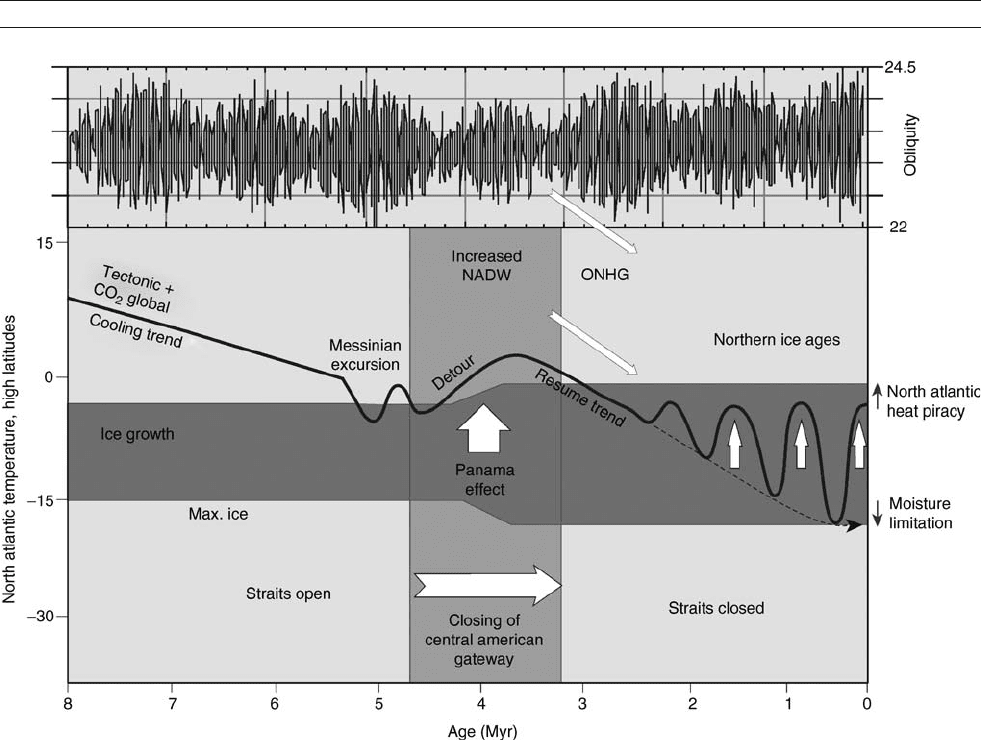
Figure Q4 Summary of the causes of the Intensification of Northern Hemisphere Glaciation (INHG). Note the detour of the cooling trend and the

expansion of the temperature range of ice growth caused by the closure of the Central American gateway. Note also the kick in obliquity that

occurs between 3.2 and 2.5 Ma and drives the continued cooling of the climate system and the INHG (adapted from Berger and Wefer, 1996).

QUATERNARY CLIMATE TRANSITIONS AND CYCLES 845

cycles. This is because the Southern Hemisphere is limited in

its response as the expansion of the ice sheets is curtailed by

the Southern Ocean around Antarctica. It was initially sug-

gested by Milankovitch ( 1949 ) that the critical factor is total

summer insolation at about 65



N, as the ice sheets must survive

the summer melting. The conventional view of glaciation is

that low summer insolation in the temperate North Hemisphere

allowed ice to survive summer and thus start to buildup on the

northern continents (Hays et al., 1976). At some point, this

expansion allowed the ice sheet to produce its own sustainable

environment, primarily by increasing the albedo, and thereby

promoting the accumulation of more ice (Figure Q5). The next

critical stage occurred when the ice sheets, particularly the

Laurentide Ice Sheet on North America, become big enough

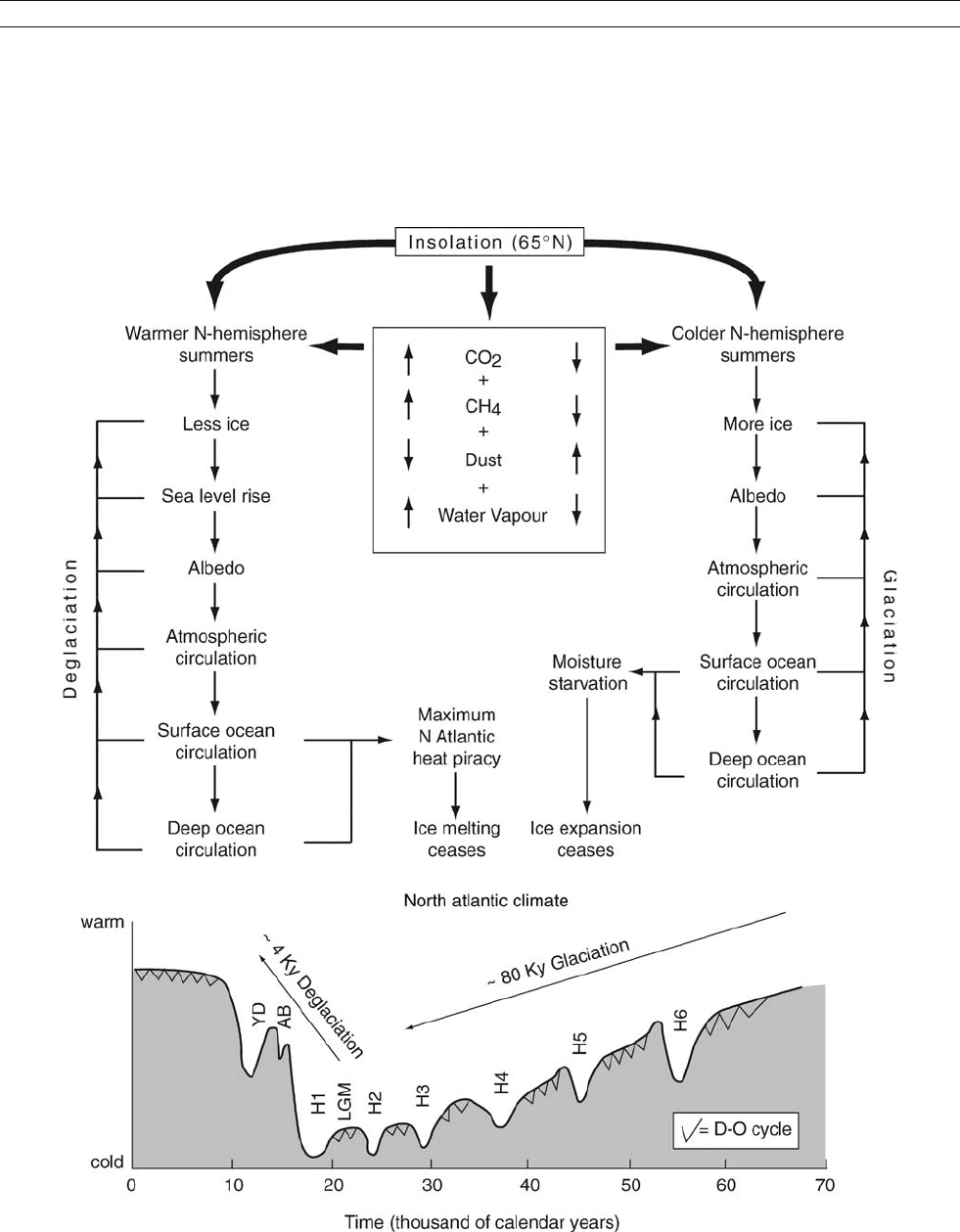
Figure Q5 Summary of the feedback mechanisms forced by insolation at 65



N that drive glaciation and deglaciation. H: Heinrich events, LGM: Last

Glacial Maximum, AB: Allerød Bølling Interstadial, YD: Younger Dryas Stadial and D-O: Dansgaard-Oeschger cycles.

846 QUATERNARY CLIMATE TRANSITIONS AND CYCLES

to deflect atmospheric planetary waves (Huybers and Tziper-

man, 2007). This changed the storm path across the North

Atlantic Ocean and prevented Gulf Stream penetration as far

north as today. This surface ocean change and increased melt-

water in the Nordic Seas and Atlantic Ocean ultimately reduced

the production of deepwater. This in turn reduced the amount

of warm water pulled northwards. All of these led to increased

cooling in the Northern Hemisphere and expansion of the ice

sheets.

There are other feedback mechanisms that also helped drive

the system towards maximum possible glacial conditions

(Raymo and Huybers, 2008). These include changes in the car-

bon cycle that reduced both atmospheric carbon dioxide and

methane. Ridgwell et al. (2003) discuss the main controls on

the carbon cycle and the possible causes of reduced glacial

atmospheric carbon dioxide. They speculate that glacial-inter-

glacial changes in atmospheric carbon dioxide may be primar-

ily driven by changes in oceanography in the Southern Ocean.

This could have altered the nutrient supply to the surface

waters, and hence surface water productivity. Dust-stimu lated

increased glacial surface water productivity would have drawn

down atmospheric carbon dioxide into the surface water to pro-

duce organic matter through photosynthesis. However, the con-

trols on the glacial-interglacial carbon cycle are still very

poorly understood. Glacial periods are also by their very nature

drier, which reduces atmospheric water vapor. For example,

Lea et al. (2000) provide clear evidence that the water vapor

production of the equatorial Pacific zone was greatly curtailed

during the last five glacial periods. CO

,CH

and water vapor

are all crucial greenhouse gases and any reduction in them

leads to general global cooling (Figure Q5), which in turn

furthers glaciation.

These feedbacks are prevented from becoming a runaway

effect by “moisture limitation.” As warm surface water is

forced further and further south, the moisture supply that is

required to build ice sheets decreases. Moreover, it is very clear

that ice sheets are naturally unstable and these feedbacks are

constantly altering direction during the whole glacial period,

hence it takes 80 ka to achieve the maximum ice extent during

the LGM and that period is characterized by rapid oscillations

such as Heinrich events and D-O cycles (see below).

The natural instability of ice sheets means that deglaciation

is much quicker than glaciation. For example, the last deglacia-

tion or Termination I, endured a maximum of 4 ka including

the brief return to glacial conditions called the Younger Dryas

period. The increase in summer 65



N insolation (e.g., Imbrie

et al., 1993) led to the initial melting of the northern ice sheets.

The resultant raised sea level then undercut the ice sheets adja-

cent to the oceans, which in turn increased sea level. This sea

level feedback mechanism was extremely rapid. Once the ice

sheets retreated then the other feedback mechanisms discussed

for glaciation reversed (see Figure Q5), leading to a massive

increase in the greenhouse gases CO

,CH

and water vapor.

These feedbacks were prevented from creating a runaway effect

by the limit of how much heat the North Atlantic could steal

from the South Atlantic to maintain the interglacial deep-water

overturning rate.

The latest data concerning the link between orbital forcing

and these feedbacks suggests that changes in the carbon cycle

lead to changes in global ice volume (Shackleton, 2000; Ridgwell

et al., 2003; Ruddiman and Raymo, 2003; Pagani et al., 2005;

Raymo and Huybers, 2008). This suggests that orbital forcing

has a direct effect on atmospheric carbon dioxide and methane,

which may drive global temperatures, and in turn change glo-

bal ice volume. Thus, the carbon cycle, instead of being a

response to glacial-interglacial cycles, could indeed be one of

the key driving forces (see Figure Q5).

The Mid-Pleistocene revolution

Debunking the eccentricity myth?

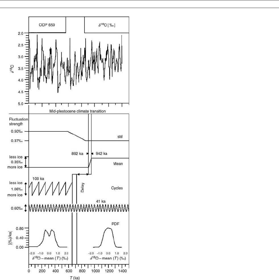
The Mid-Pleistocene Revolution (MPR) is the term used to

denote the marked prolongation and intensification of the glo-

bal glacial-interglacial climate cycles which occurred between

900 and 650 ka (Berger and Jansen, 1994). Prior to the MPR,

since at least the intensification of Northern Hemisphere glacia-

tion (2.75 Ma), global climate appears to have responded to

obliquity variations (Imbrie et al., 1992), i.e., the glacial-intergla-

cial cycles occurred with a frequency of 41 kyr. After about

800 ka, glacial-interglacial cycles became more pronounced

and occurred with a frequency of approximately 100 ka. The

MPR, therefore, marks a dramatic sharpening of the contrast

between warm and cold periods. Mudelsee and Stattegger

(1997) used advanced methods of time-series analysis to

review the deep-sea evidence spanning the MPR and summar-

ized the salient features (Figure Q6). The first transition

occurred between 942 and 892 ka when global ice volume sig-

nificantly increased. However, the 41 ka climate forcing contin-

ued. This situation persisted until about 650–725 ka when the

climate system entered a bi-modal phase and the strong 100 ka

climate cycles began (Mudelsee and Stattegger, 1997).

Imbrie et al. (1993) called the MPR the “100 ka problem,”

as the eccentricity signal is by far the weakest of the orbital

parameters. Hence, it has been assumed that there must have

been a change from a linearly to a non-linearly forced climate

system (Imbrie et al., 1992, 1993). Many different theories

have thus been postulated to produce this critical non-linear

transition, including: critical size of the Northern Hemisphere

ice sheets, global cooling trend, erosion of regolith beneath

the Laurentide Ice Sheet, o rbital inclination, Greenland-

Scotland submarine ridge and carbon cycle and atmospheric

(see Maslin and Ridgwell, 2005 for detailed references).

There are a number of problems with associating the 100 ka

cycles with eccentricity. The first is that eccentricity has spec-

tral peaks at 95 ka, 125 ka and 400 ka. The spectral analysis

of benthic foraminifera oxygen isotopes (SPECMAP) – a

proxy for global ice volume – shows a consistent single peak

of 100 ka (Maslin and Ridgwell, 2005). However, the lengths

of the last 8 glacial-interglacial cycles vary from 87 to 119 ka,

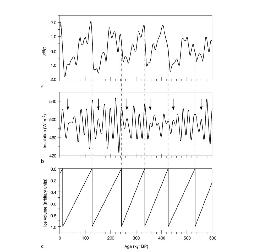
averaging about 100 ka. Ridgwell et al. (1999) demonstra-

ted that this strong 100 ka peak could not be produced by

eccentricity, but rather by a simple saw-tooth pattern based on

a long glaciation period followed by a short deglaciation

(Figure Q7). This suggests that the 100 ka cycle seen in the

ice volume records is dominated by deglaciations that occur

every 100 ka after the MPR, on average. Note that summer

insolation at 65



N is also strongly influenced by precession;

hence, the saw-toothed pattern of rapid deglaciation occurs

every fourth or fifth precessional cycle over the last 600 ka.

A similar saw-tooth pattern can be produced from obliquity

using every second or third cycle (Ridgwell et al., 1999;

Huybers and Wunsch, 2005; Raymo et al., 2006; Raymo and

Huybers, 2008), but the spectral analysis does not match the

global ice volume signal as well (Ridgwell et al., 1999; Maslin

and Ridgwell, 2005). Models have also been used to re-create

the 100 ka cycle and the most successful is the LLN 2D model,

QUATERNARY CLIMATE TRANSITIONS AND CYCLES 847

which combines orbital forcing with atmospheric carbon diox-

ide. Hence, the keys to the MPR are precession and atmo-

spheric carbon dioxide. Ridgwell et al (1999) suggested that

the episodic occurrence of unusually low maxima in Northern

Hemisphere summer insolation is the critical factor controlling

subsequent deglaciation. Ruddiman (2003) furthermore sug-

gests that both precession and obliquity affect the concentration

of the greenhouse gases carbon dioxide and methane, and this

combined influence results in the strong 100 ka cycle. This

means that all three orbital periodicities are involved and the

MPR is not a simple non-linear amplification of eccentricity.

In effect, this new research from the study of the MPR suggests

that it is very hard to get the global climate system out of a gla-

cial or near-glacial condition. Deglaciation can only occur

when the climate system has been allowed to reach maximum

glaciation by the previous low maxima in Northern Hemi-

sphere summer insolation, for example during the LGM. The

following precessionally driven summer maxima pushes the

climate system too far and it overshoots the mild glacial (e.g.,

oxygen isotope stage 3 to 5a) type climate, entering an intergla-

cial period.

The dominance of precession leads to another problem, the

assumption of a linear response of the climate system to obli-

quity prior to MPR (Imbrie et al., 1992), as the insolation

records for 2.5–1 Ma for the temperate regions are very similar

to the period after 1 Ma, i.e., dominated by precession. Raymo

and Nisancioglu (2003) suggest another solution to the obli-

quity problem: the MPR is a switch from an obliquity-driven

latitudinal heat gradient system to a precessional-driven degla-

cial system. In contrast Raymo et al. (2006) and Raymo and

Huybers (2008) suggested that prior to the MPR both the

Northern Hemisphere and Antarctic ice sheets are responding

to precession; but because they are 180



out of phase the pre-

cessional component cancels out leaving a dominant obliquity

signal. After the MPR the dominance of the Northern Hemi-

sphere ice sheet is such that Northern Hemisphere precession

dominates global climate.

Millennial-climate cycles

Heinrich events

Heinrich events are intense and quasi-periodic ice-rafting

pulses that are thought to originate primarily from the Laurentide

Ice Sheet (e.g., Ruddiman, 1977; Heinrich, 1988; Bond et al.,

1992; Maslin et al., 1995). These events occurred against the

general background of unstable glacial climate, and represent

the brief expression of the most extreme glacial conditions

around the North Atlantic. Heinrich events are evident in the

Greenland ice cores as a further 3–6



C drop in temperature

from the already cold glacial climate (Bond et al., 1993;

Dansgaard et al., 1993). These events have been found to have

a global impact with evidence for coeval climate changes from

as far a field as: South America, North Pacific, Santa Barbara

Basin, Arabian Sea, China, South China Sea, and Sea of Japan

(e.g., reviewed in Maslin et al., 2001). Around the North Atlantic,

much colder conditions prevailed in both North America and

Europe, while huge armadas of melting icebergs reduced sea

surface temperatures in the North Atlantic Ocean by another

1–2



C and reduced the surface salinity by up to 4% (Chapman

and Maslin, 1999; Rashid and Boyle, 2007).

Detailed studies of the sequence of events in ocean sediments

and ice cores show that Heinrich events occurred on an average

of 7,200  2,400 calendar years in the time interval between

about 70 and 10.5 ka. In between the Heinrich events, much

higher frequency, smaller amplitude events occurred about every

1,500 years, which are referred to as Dansgaard-Oeschger events

or cycles (Dansgaard et al., 1993;Bondetal.,1997). Heinrich

events may in fact be just super Dansgaard-Oeschger events.

(see Dansgaard-Oeschger cycles; Heinrich events).

Dansgaard-Oeschger cycles

Dansgaard-Oeschger (D-O) cycles were first identified in the

Greenland ice core records (Dansgaard et al., 1993). A succession

Figure Q6 Detailed breakdown of the Mid-Pleistocene Revolution

(after Mudelsee and Stattegger, 1997), demonstrating a delay of 200 ka

between the significant increase in global ice volume and the start of

the 100 ka glacial-interglacial cycles.

848 QUATERNARY CLIMATE TRANSITIONS AND CYCLES

of short lived “warm” events or Greenland interstadials (GIS)

characterize the ice core records of the last glacial episode

and are numbered down from the “Bølling” as GIS 1 to GIS

24 at 105 ka. The D-O stadials or cold sections of the D-O

cycle have been found in the ice rafting records of the North

Atlantic (e.g., Bond and Lotti, 1995). These stadials are char-

acterized by increased meltwater and ice-rafted debris originat-

ing from Iceland and East Greenland. These D-O cycles have a

frequency of 1,479  532 years, and seem to persist into the

Holocene interglacial as well as occurring during earlier glacial

and interglacial stages (Bond et al., 2001). A precise time-

scale for the duration and sequence of these millennial-scale

climate events is uncertain, though the events themselves do

not appear to have lasted longer than a few centuries. Further-

more, the transitions marking the beginnings and ends of each

Heinrich and D-O event are particularly rapid, probably lasting

no more than a few decades, indicating that climate responded

in a step-like series of jumps to whatever driving mechanism

initiated them.

Possible causes of the Heinrich events and

Dansgaard-Oeschger cycles

There are a number of possible causes suggested for these mil-

lennial climate cycles, including the theory that they are due

to stochastic resonance (Alley et al., 2001). Although none

Figure Q7 (a) SPECMAP stacked d

O composite, (b) insolation for June 21 65



N showing the quasi-periodic insolation maxima of unusually low

strength (shown by arrows) preceding glacial-interglacial terminations by one precessional cycle in each case and (c) sawtooth artificial ice volume

signal.

QUATERNARY CLIMATE TRANSITIONS AND CYCLES 849

of these theories is conclusive, the major ones are summari-

zed below.

Internal ice sheet failure

MacAyeal (1993a,b) suggested that the Heinrich event iceberg

surges were caused by internal instabilities of the Laurentide

Ice Sheet. This ice sheet rested on a bed of soft unconsolidated

sediment, which, when it was frozen, did not deform and

behaved like concrete, so that it would have been able to

support the weight of the growing ice sheet. As the ice sheet

expanded, the geothermal heat from within the Earth’s crust,

together with heat released from friction of ice moving over

ice was trapped by the insulating effect of the overlying ice.

This “duvet” effect allowed the temperature of the sediment

to increase until a critical point when it thawed. When this

occurred, the sediment became soft, and thus lubricated the

base of the ice sheet, causing a massive outflow of ice through

the Hudson Strait into the North Atlantic. This, in turn, led to

sudden loss of ice mass, which then reduced the insulating

effect and led to re-freezing of the basal ice and sediment

bed, at which point the ice reverted to a slower build-up and

outward movement. According to MacAyeal (1993a,b), this

system of progressive ice build-up, melting and surge, followed

by renewed build-up, has an approximate periodicity of 7,000

years, which compares well with the interval between the last

six Heinrich events, which is on average 7,200  2,400 calen-

dar years. However, different ice sheets may have had different

binge-purge times, thus the Fenno-Scandinavian, Greenland

and Icelandic Ice Sheets would have surged with different per-

iodicities. An alternative suggestion is that D-O events are

caused by the more frequent regular failure of the European

and Greenland Ice Sheet, while the larger, more infrequent

Heinrich events are caused by collapse of the Laurentide

Ice Sheet.

Sea level connection between Heinrich and D-O events

The second theory is that sea level rises induced by the 1,500-

year D-O cycles undercuts and thus destabilizes the Laurentide

Ice Sheets, triggering a much larger Heinrich event. The peri-

odicities are such that a Heinrich event occurs for every fifth

D-O cycle. Support for this theory comes from the detailed

analysis of the sources of ice-rafted material in the Heinrich

layers. From the detailed breakdown of H1, H2, H4 and H5,

it has been shown that European ice-rafted debris was depos-

ited in the North Atlantic up to 1,500 years before the Laurentide

material (e.g., Grousset et al., 2000). This theory, however,

does not explain what causes the Dansgaard-Oeschger cycles,

since they occur with a similar frequency during both glacial

and interglacial periods.

Bipolar climate seesaw

Ice core data from Greenland and Antarctica show an out-of-

phase relationship in glacial millennial-scale climate cycles

for the North and Southern Hemisphere (Blunier et al., 1998),

see Figure Q8. It has been suggested that this so-called bipolar

climate seesaw can be explained by alternating meltwater

events in the North Atlantic and Southern Ocean. Each melt-

water event would change the relative amount of deepwater

formation in the two hemispheres and the resulting direction of

inter-hemispheric “heat piracy” (Figure Q8; Seidov and Maslin,

2001; Seidov et al., 2001; see Thermohaline circulation). The

bipolar seesaw model suggested by Maslin et al. (2001) could

be self-sustaining with meltwater events in either hemisphere

triggering a chain of climate changes that eventually causes a

meltwater event in the opposite hemisphere by switching the

direction of the hemispheric heat exchange (Figure Q9). The

advantage of this theory is that it can explain D-O cycles during

both glacial and interglacial periods.

External forcing

Heinrich (1988) originally suggested that ice-rafting events

could be forced by harmonics of orbital parameters, as their

quasi-cyclicity is on the order of 10 kyr. However, it now

seems that the periodicity shortens through a glacial period

starting at 13 ka and decreasing to 7 ka. With the discovery that

Heinrich events were part of the more frequent D-O cycles and

that both hemispheres respond asynchronously, it is unlikely

that longer-term orbital forcing (minimum 10 kyr) could be

the cause. Hence, until recently it was thought these millennial

events were internally and not externally, forced. The latest

development in this area is a study showing a significant corre-

lation between drift-ice deposited material in the North Atlantic

and the production of both

C and

Be in the atmosphere over

the last 12,000 years (Bond et al., 2001). Bond et al. suggest

that the production of both

C and

Be indicates millennial-

scale variations in solar output, which may have caused the

D-O climate cycles. They further postulate that amplification

of relatively weak solar changes was due to the Arctic-Nordic

Sea’s sensitivity to changes in surface-water salinity. Hence,

increased freshening of this region would reduce the North

Atlantic Deep Water (NADW) and thus transmit the solar influ-

ence globally. However, a number of problems remain with the

millennial-scale solar output theory, the most important being

how the extremely small solar output variations are translated

into regional and global climate changes of over 2



C. The

debate about solar forcing on Holocene climate records and

its application to glacial periods continues (e.g., Braun et al.,

2005; Holocene climates).

Last glacial-interglacial transition (LGIT)

The nature of the LGIT

The last glacial-interglacial transition (LGIT, ca. 14–9

BP) was characterized by a series of extremely abrupt cli-

matic changes (e.g., Alley and Clark, 1999; Lowe and Walker,

2000; Stocker, 2003). These abrupt climate shifts are found in

earlier glacial terminations and therefore seem to be part of

the natural climate variability associated with this type of tran-

sition. The two most prominent features are rapid warming at

14.7 k GRIP ice-core years

BP (the start of the “Bølling” epi-

sode) and the well-known period of severe cooling referred to

as the Younger Dryas Stadial, dated to between 12.7 and 11.5

BP in GRIP ice-core years. These features are easily recog-

nizable in a wide range of proxy records from sites throughout

the Northern Hemisphere (e.g., Alley and Clark, 1999). There

is also a growing body of evidence that suggests that parts of

the Southern Hemisphere may have experienced a broadly

similar sequence of climatic events, including parts of South

America and New Zealand.

According to the GRIP and GISP2 ice-core records (e.g.,

Dansgaard et al., 1993; Alley and Clark, 1999), the sequence

of events during the last glacial-interglacial transition were far

more abrupt than had been assumed from prior interpretations

based on continental and marine stratigraphical records.

850 QUATERNARY CLIMATE TRANSITIONS AND CYCLES

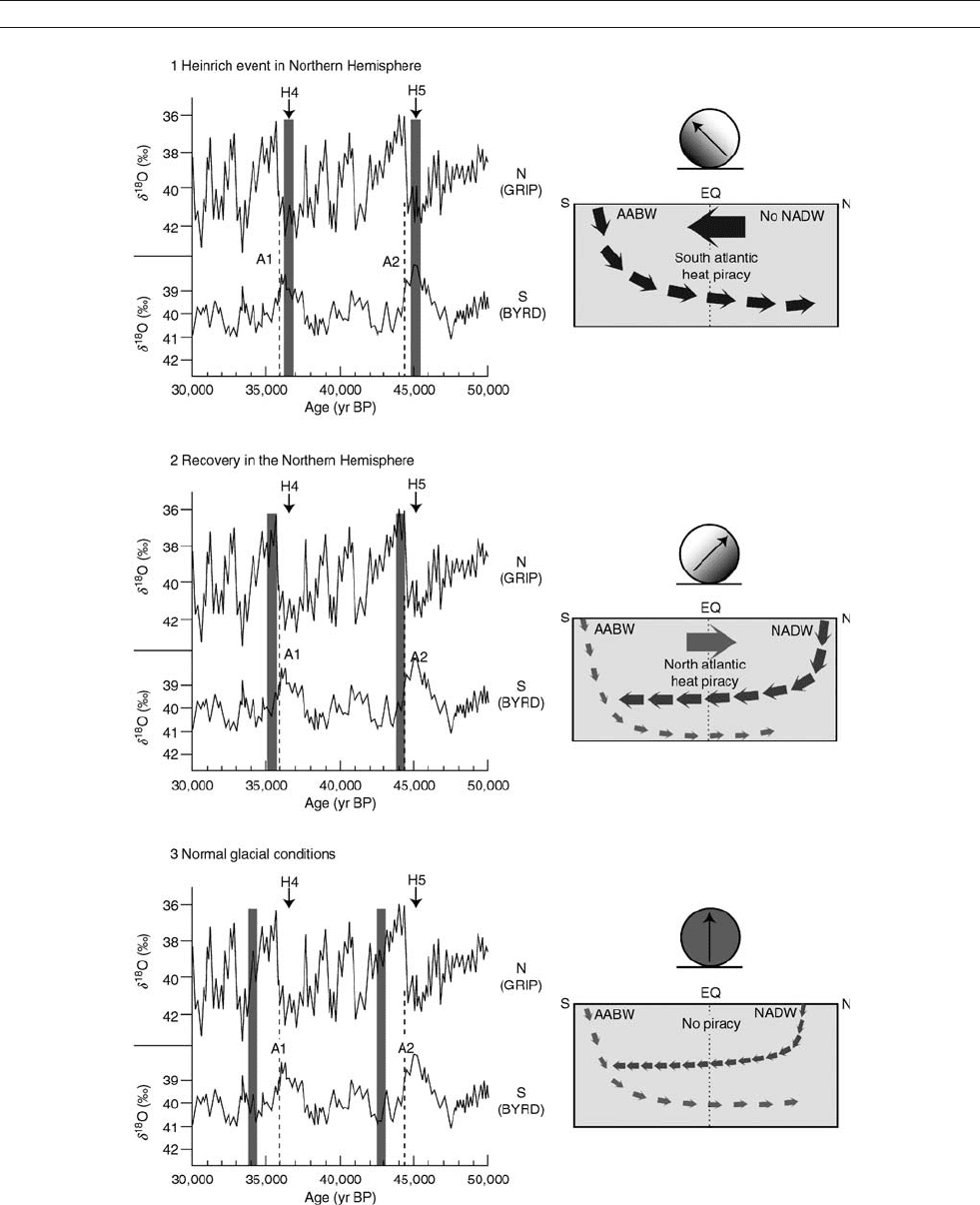
Figure Q8 Left: Greenland (GRIP) and Antarctic (Byrd) ice core d

O temperature proxy records on the age models generated by Blunier et al.

(1998). Three time slices are illustrated with solid bars; (1) Heinrich event, (2) Northern Hemisphere climate recovery post-Heinrich event, and

(3) Normal glacial conditions. Right: Schematic view of oscillating meridional ocean overturning and associated regimes of heat transport in the

Atlantic Ocean, showing which hemisphere controls deepwater circulation and thus inter-hemispheric heat transport (adapted from Maslin

et al., 2001 and Seidov et al., 2001).

QUATERNARY CLIMATE TRANSITIONS AND CYCLES 851