Patrick F. Dunn, Measurement, Data Analysis, and Sensor Fundamentals for Engineering and Science, 2nd Edition

Подождите немного. Документ загружается.

306 Measurement and Data Analysis for Engineering and Science

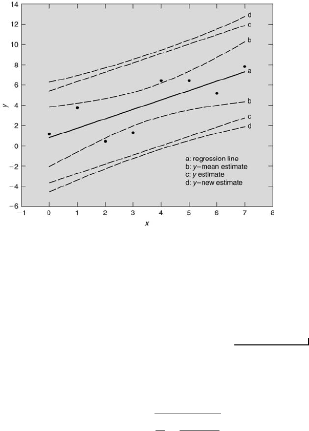
FIGURE 8.4

Various conﬁdence intervals for linear regression estimates.

analysis. Then estimate at 95 % conﬁdence the values of the true intercept and the

true slope.

Solution: The best-ﬁt relation is y = 0.96 + 1.02x for N = 5 with S

= 0.12,

= 10, ¯x = 3, and t

3,95

= 3.1824. This yields α = 0.96 ± 0.40 (95 %) and β =

1.02 ± 0.12 (95 %).

The values of some other useful quantities also can be estimated [5], [6],

[7]. The estimate of the sample mean value of a large number of y

values

for a given value of x

, denoted by ¯y

, and also known as the mean response,

¯y

= y

± t

N−2,P

− ¯x)

. (8.28)

Note that the greater the diﬀerence between x

and ¯x, the greater the un-

certainty in estimating ¯y

. This leads to conﬁdence intervals that are hy-

perbolic, as shown in Figure 8.4 by the curves labeled b (based upon 95 %

conﬁdence), that are positioned above and below the regression line labeled

by a. The conﬁdence interval is the smallest at x = ¯x. Also, because of

the factor t

ν,P

, the conﬁdence interval width will decrease with decreasing

percent conﬁdence.

The range within which a new y value, y

, added to the data set will be

for a new value x

Regression and Correlation 307

= y

± t

N−2,P

1 +

− ¯x)

. (8.29)

This interval is marked by the hyperbolic curves labeled d (based upon

95 % conﬁdence). Note that the hyperbolic curves are farther from the

regression line for this case than for the mean response case. This is because

Equation 8.29 estimates a single new value of y, whereas Equation 8.28

estimates the mean of a large number of y values.

Finally, the range within which a y

value probably will be, with respect

to its corresponding y

value, is

= y

± t

ν,P

, (8.30)

where t

ν,P

denotes the precision interval. This expression establishes

the conﬁdence intervals that always should be plotted whenever a regression

line is present. Basically, Equation 8.30 deﬁnes the limits within which P

percent of a large number of measured y

values will be with respect to

the y

value for a given value of x

. Its conﬁdence intervals are denoted

by the lines labeled c (based upon 95 % conﬁdence) which are parallel to

the regression line. Equation 8.30 also can be used for a higher mth-order

regression ﬁt to establish the conﬁdence intervals. This is provided that ν

is determined by ν = N − (m + 1) and that the general expression for S

given in Equation 8.25 is used.

Several useful inferences can be drawn from Equation 8.30. For a ﬁxed

number of measurements, N, the extent of the precision interval increases as

the percent conﬁdence is increased. The extent of the precision interval must

be greater if more conﬁdence is required in the estimate of y

. For a given

conﬁdence, as N is increased the extent of the precision interval decreases.

A smaller precision interval is required to estimate y

if a greater number of

measurements is acquired.

Example Problem 8.4

Statement: For the set of [x,y] data pairs [0.00, 1.15; 1.00, 3.76; 2.00, 0.41; 3.00,

1.30; 4.00, 6.42; 5.00, 6.42; 6.00, 5.20; 7.00, 7.87] determine the linear best-ﬁt relation

using least-squares regression analysis. Then estimate at 95 % conﬁdence the intervals

of ¯y

, y

, and y

according to Equations 8.28 through 8.30 for x = 2.00.

Solution: From Equation 8.28 it follows directly that ¯y

= 2.68 ± 1.93. That is,

there is a 95 % chance that the mean value of a large number of measured y

values

for x = 2.00 will be within ±1.93 of the y

value of 2.68. Further, from Equation 8.29,

= 2.68 ± 4.95, which implies that there is a 95 % chance that a new measurement

of y for x = 2.00 will be within ±4.95 of 2.68. Finally, from Equation 8.30, y

= 2.68

± 4.56. The conﬁdence intervals for this data set for the range 0 ≤ x ≤ 7 are shown in

Figure 8.4.

Another conﬁdence interval related to the regression ﬁt can be estab-

lished for the estimate of a value of x for a given value of y. This situation

308 Measurement and Data Analysis for Engineering and Science

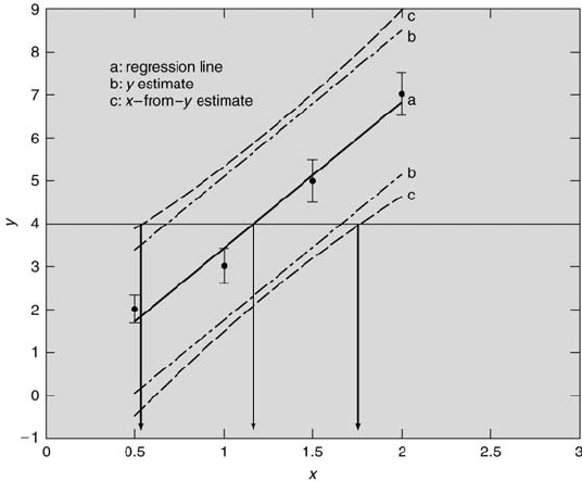
FIGURE 8.5

Regression ﬁt with relatively large sensitivity.

is encountered when a calibration curve is used to determine unknown x

values. Figures 8.5 and 8.6 each display a linear regression ﬁt of the data

(labeled by a) along with two diﬀerent conﬁdence intervals for P = 95 %. In

addition to the usual estimate of the range within which a y

value will be

with respect to its calculated value (labeled by b), there is another estimate,

the x -from-y estimate with its conﬁdence interval (labeled by c). This new

estimate’s conﬁdence interval should be greater in extent than that for the

y estimate. This is because additional uncertainties arise when the best ﬁt

is used to project from a chosen y value back to an unknown x value.

The conﬁdence interval for the estimate of x from y is represented by

hyperbolic curves. The uncertainty forming the basis of this conﬁdence in-

terval results from three diﬀerent uncertainties associated with y and the

best-ﬁt expression: from the measurement uncertainty in y, from the uncer-

tainty in the true value of the intercept, and from the uncertainty in the true

value of the slope. The latter two result from determining the regression ﬁt

based upon a ﬁnite amount of data. In essence, the hyperbolic curves can

be viewed as bounds for the area within which all possible ﬁnite regres-

sion ﬁts with their standard y-estimate conﬁdence intervals are contained.

When one projects from a chosen y value back to the x -axis, one does not

know upon which regression ﬁt the projected x value is based. The chosen

y value could have resulted from an x value diﬀerent than the one used to

establish the ﬁt. This new conﬁdence interval accounts for this. The three

Regression and Correlation 309

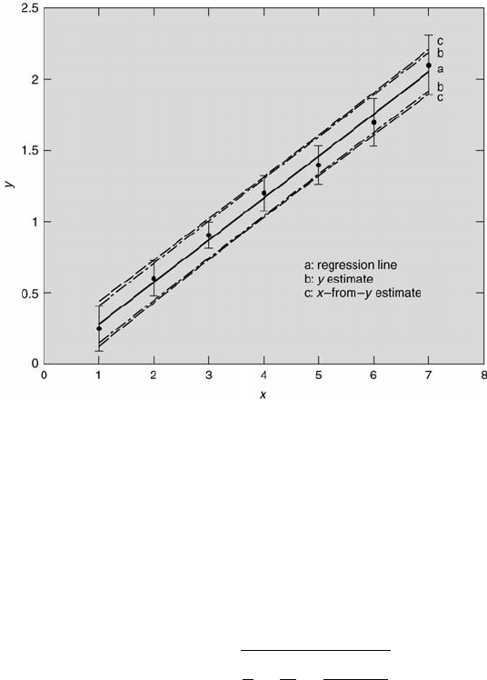
FIGURE 8.6

Regression ﬁt with relatively small sensitivity.

contributory uncertainties cannot be combined in quadrature to yield the

ﬁnal uncertainty because the intercept and slope uncertainties are not sta-

tistically independent from one another. So, a more rigorous approach must

be taken to determine this conﬁdence interval. This was done by Finney [8],

who established this conﬁdence interval to be

y = y

± t

ν,P

(x − ¯x)

, (8.31)

where n denotes the number of replications of y measurements for a partic-

ular value of x (n = 1 for the examples shown in Figures 8.6 and 8.5).

A comparison of Figures 8.5 and 8.6 reveals several important facts.

When the magnitude of the uncertainty in y is relatively small, the conﬁ-

dence limits are closer to the regression line. When there is more scatter in

the data, both intervals are wider. Fewer [x,y] data pairs result in a rela-

tively larger diﬀerence between the conﬁdence limits. The sensitivity of y

with respect to x (the slope of the regression line) plays an important role

in determining the level of uncertainty in x in relation to the x-from-y con-

ﬁdence interval. Lower sensitivities result in relatively large uncertainties in

x. For example, the uncertainty range in x for a value of y = 4.0 in Figure

8.5 is from approximately 0.53 to 1.76, as noted by the arrows in the ﬁgure,

310 Measurement and Data Analysis for Engineering and Science

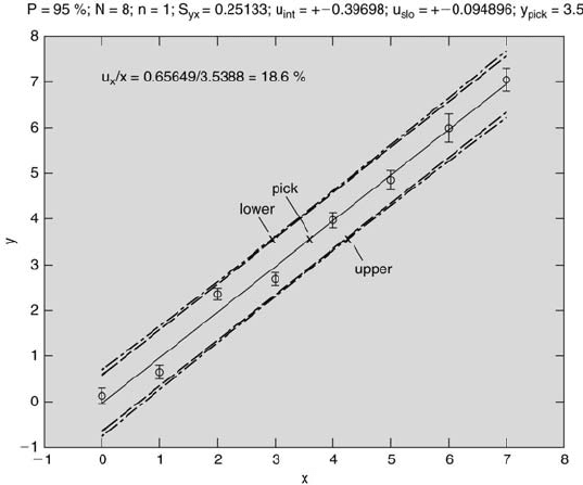
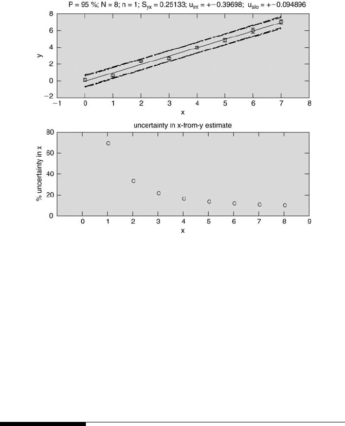
FIGURE 8.7

Regression ﬁt with indicated x-from-y estimate uncertainty.

for a calculated value of x = 1.18. Note that the range of this uncertainty

is not symmetric with respect to the calculated value of x.

The M-ﬁle caley.m performs a linear least-squares regression analysis

on a set of [x, y, ey] data pairs (where ey is the measurement error of y)

and plots the regression ﬁt and its associated conﬁdence intervals, as given

by Equations 8.30 and 8.31. This M-ﬁle was used to generate Figures 8.5

and 8.6. The M-ﬁle caleyII.m also determines the range in the x-from-y

estimate for a user-speciﬁed value of y, as shown in Figure 8.7. The M-ﬁle

caleyIII.m extends this type of analysis farther by determining the percent

uncertainty in the x-from-y estimate for the entire range of y values. It plots

the standard regression ﬁt with the data and also the x-from-y estimate

uncertainty versus x. The two resulting plots are shown in Figure 8.8.

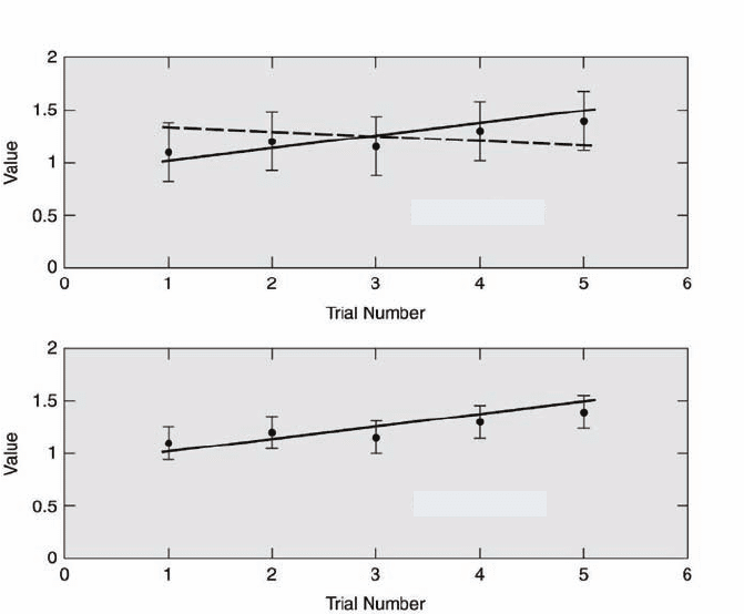
Caution should be exercised when claims are made about trends in the

data. Any claim must be made within the context of measurement uncer-

tainty that is assessed at a particular conﬁdence level. An example is illus-

trated in Figure 8.9. The same values of ﬁve trials are plotted in each of

the two ﬁgures. The trend in the values appears to increase with increasing

trial number. In the top ﬁgure, the error bars represent the measurement

uncertainty assessed at a 95 % level of conﬁdence. The solid line suggests an

increasing trend, whereas the dotted line implies a decreasing trend. Both

claims are valid to within the measurement uncertainty at 95 % conﬁdence.

In the bottom ﬁgure, the error bars represent the measurement uncertainty

Regression and Correlation 311

FIGURE 8.8

Regression ﬁt and x-from-y estimate uncertainty.

assessed at a 68 % level of conﬁdence. It is now possible to exclude the claim

of a decreasing trend and support only that of an increasing trend. This,

however, has been done at the cost of reducing the conﬁdence level of the

claim. In fact, if the level of conﬁdence is reduced even further, the claim of

an increasing trend cannot be supported. Thus, a speciﬁc trend in compar-

ison with others can only be supported through accurate experimentation

in which the error bars are small at a high level of conﬁdence.

8.7 Linear Correlation Analysis

It was not until late in the 19th century that scientists considered how to

quantify the extent of the relation between two random variables. Francis

Galton in his landmark paper published in 1888 [16] quantitatively deﬁned

the word co-relation, now known as correlation. In that paper he presented

for the ﬁrst time the method for calculating the correlation coeﬃcient and

its conﬁdence limits. He was able to correlate the height (stature) of 348

adult males to their forearm (cubit) lengths. This data is presented in Table

8.1. Galton designated the coeﬃcient by the symbol r, which “measures the

312 Measurement and Data Analysis for Engineering and Science

95 % confidence

68 % confidence

FIGURE 8.9

Data trends with respect to uncertainty.

closeness of co-relation.” This symbol still is used today for the correlation

coeﬃcient.

Galton purposely presented his data in a particular tabular form, as

shown in Table 8.1. In this manner, a possible co-relation between stature

and cubit became immediately obvious to the reader, as indicated by the

larger numbers along the table’s diagonal. All that was left after realizing

a co-relation was to quantify it. Galton approached this in an ad hoc man-

ner by computing the mean value for each row (the mean cubit length for

each stature) as well as the overall mean (the mean cubit length for all

statures). He then expressed this data in terms of standard units (the num-

ber of probable measurement error units from the overall mean). He plotted

the standardized unit values for each row (the standardized cubit lengths)

versus the standardized unit value of the row (the standardized stature).

This yielded the regression of cubit length upon stature. He followed a sim-

ilar approach to determine the regression of stature upon cubit length by

interchanging the rows and columns of data. He then established the com-

posite best linear ﬁt by eye and approximated the slope’s value to be equal

Regression and Correlation 313

16.5

17.0

17.5

18.0

18.5

19.0

19.5

C <

< C <

< C

16.5

17.0

17.5

18.0

18.5

19.0

19.5

S > 71

71 > S > 70

70 > S > 69

69 > S > 68

68 > S > 67

67 > S > 66

66 > S > 65

65 > S > 64

64 > S

TABLE 8.1

Galton’s data of stature (S) versus cubit (C) length [16] (units of inches).

to 0.8, which was the regression coeﬃcient. This approach was formalized

later by the statisticians Francis Edgeworth and Karl Pearson.

But what exactly is the correlation coeﬃcient and how can it be calcu-

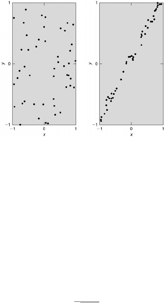
lated? This relates to the general process of correlation analysis. In this

section only linear correlation analysis is considered. In general, two ran-

dom variables, x and y, are correlated if x ’s values can be related to the y’s

values to some extent. In the left graph of Figure 8.10, the variables show

no correlation, whereas in the right graph, they are correlated moderately.

The extent of linear dependence between x and y is quantiﬁed through

the correlation coeﬃcient. This coeﬃcient is related to the population vari-

ances of x and y, σ

and σ

, and the population covariance, σ

. The

population correlation coeﬃcient is deﬁned as

ρ ≡

√

, (8.32)

where

≡ E[(x − x

)(y − y

)] = E[xy] − x

, (8.33)

≡

E[(x − x

)

], (8.34)

and

≡

E[(y − y

)

]. (8.35)

E[ ] denotes the expectation or mean value of a quantity, which for any

statistical parameter q raised to a power m involving N discrete values is

E[q

] ≡ lim

N→∞

i=1

. (8.36)

314 Measurement and Data Analysis for Engineering and Science

FIGURE 8.10

Uncorrelated and correlated data.

Two parameters, q and r, are statistically independent when

E[q

· r

] = E[q

] · E[r

], (8.37)

where m and n are powers.

The covariance is the mean value of the product of the deviations of x

and y from their true mean values. The population correlation coeﬃcient is

simply the ratio of the population covariance to the product of the x and

y population variances. It measures the strength of the linear relationship

between x and y. When ρ = 0, x and y are uncorrelated, which implies

that y is independent of x. When ρ = ±1, there is perfect correlation, where

y = a ± bx for all [x,y] pairs.

The sample correlation coeﬃcient, r, is an estimate of the pop-

ulation correlation coeﬃcient, ρ. That is, the population correlation

coeﬃcient can be estimated but not determined exactly because a sample

is ﬁnite and a population is inﬁnite. The sample correlation coeﬃcient is

deﬁned in a manner analogous to Equation 8.32 as

r =

. (8.38)

Squaring both sides of this equation, substituting Equation 8.18 for the

slope of the regression line, and then taking the square root of both sides,

Equation 8.38 becomes

Regression and Correlation 315

b = r

. (8.39)

Thus, the slope of the regression ﬁt equals the linear correlation coeﬃcient

times a scale factor. The scale factor is simply the square root of the ratio

of the the spread of the y values to the spread of the x values. So, b and r

are related closely, but they are not the same.

Using Equations 8.15, 8.16, and 8.17, Equation 8.38 can be rewritten as

r =

i=1

− ¯x)(y

− ¯y)

i=1

− ¯x)

i=1

− ¯y)

. (8.40)

Equation 8.40 is known as the product-moment formula, which auto-

matically keeps the proper sign of r. From this, r is calculated directly from

the data without performing any regression analysis. It is evident from both

of the above equations that r is a function, not only of the speciﬁc x

and

values, but also of N . This point will be addressed shortly.

Example Problem 8.5

Statement: The Center on Addiction and Substance Abuse at Columbia University

conducted a study on college-age drinking. They reported the following average drinks

per week (DW) of alcohol consumption in relation to the average GPA (grade point

average) for a large population of college students: 3.6, A; 5.5, B; 7.6, C; 10.6, D or

F. Using an index of A = 4, B = 3, C = 2, and D or F = 0.5, determine the linear

best-ﬁt relation and the value of the linear correlation coeﬃcient.

Solution: Using the M-ﬁle plotfit.m, a linear relation with r = 0.99987 and GP A

= 5.77 − 0.50DW can be determined for the range of 0 ≤ GP A ≤ 4. These results are

presented in Figure 8.11.

A more physical interpretation of r can be made by examining the quan-

tity r

, which is known as the coeﬃcient of determination. Note that r

given by Equation 8.38 says nothing about the relation that best-ﬁts x and

y. It can be shown [5] that

SSE = S

(1 − r

) = SST (1 − r

). (8.41)

From Equations 8.22 and 8.41, it follows that

= 1 −

SSE

SSR

. (8.42)

Equation 8.42 shows that the coeﬃcient of determination is the ratio

of the explained squared variation to the total squared variation. Because

SSE and S

are always nonnegative, 1 − r

≥ 0. So, the coeﬃcient of

determination is bounded as 0 ≤ r

≤ 1. It follows directly that −1 ≤ r ≤ 1.