Patrick F. Dunn, Measurement, Data Analysis, and Sensor Fundamentals for Engineering and Science, 2nd Edition

Подождите немного. Документ загружается.

296 Measurement and Data Analysis for Engineering and Science

8.1 Chapter Overview

This chapter introduces two important areas of data analysis: regression

and correlation. Regression analysis establishes a mathematical relation

between two or more variables. Typically, it is used to obtain the best ﬁt

of data with an analytical expression. Correlation analysis quantiﬁes the

extent to which one variable is related to another, but it does not establish

a mathematical relation between them. Statistical methods can be used to

determine the conﬁdence levels associated with regression and correlation

estimates.

We begin this chapter by considering the least-squares approach to re-

gression analysis. This approach enables us to obtain a best-ﬁt relation

between variables. We focus on linear regression analysis ﬁrst. The sta-

tistical parameters that are used to characterize regression are introduced

next. Then we consider regression analysis as applied to experiments along

with their associated uncertainties and conﬁdence limits. We further exam-

ine correlation analysis by considering how a random variable is correlated

with itself and with another random variable. Finally, we examine extended

methods, including higher-order regression analysis and multi-variable linear

analysis.

8.2 Least-Squares Approach

Toward the end of the 18th century scientists faced an interesting problem.

This was how to ﬁnd the best agreement between measurements and an

analytical model that contained the measured variables, given that repeated

measurements were made, but with each containing error. Jean-Baptiste-

Joseph Delambre (1749-1822) and Pierre-Fran¸cois-Andr´e M´echain (1744-

1804) of France, for example [1] and [2], were in the process of measuring

a 10

◦

arc length of the meridian quadrant passing from the North Pole to

the Equator through Paris. The measure of length for their newly proposed

Le Syst`eme International d’Unit´es, the meter, would be deﬁned as 1/10 000

000 the length of the meridian quadrant. So, the measured length of this

quadrant had to be as accurate as possible.

Because it was not possible to measure the entire length of the 10

◦

arc,

measurements were made in arc lengths of approximately 65 000 modules

(1 module

∼

12.78 ft). From these measurements, an analytical expression

involving the arc length and the astronomically determined latitudes of each

of the arc’s end points, the length of the meridian quadrant was determined.

The solution essentially involved solving four equations containing four mea-

sured arc lengths with their associated errors for two unknowns, the elliptic-

Regression and Correlation 297

ity of the earth and a factor related to the diameter of the earth. Although

many scientists proposed diﬀerent solution methods, it was Adrien-Marie

Legendre (1752-1833), a French mathematician, who arrived at the most ac-

curate determination of the meter using the method of least squares, equal

to 0.256 480 modules (∼ 3.280 ft). Ironically, it was the more politically

astute Pierre-Simon Laplace’s (1749-1827) value of 0.256 537 modules (∼

3.281 ft) based upon a less accurate method that was adopted as the basis

for the meter. Current geodetic measurements show that the quadrant from

the North Pole to the Equator through Paris is 10 002 286 m long. This

renders the meter as originally deﬁned to be in error by 0.2 mm or 0.02 %.

Legendre’s method of least squares, which originally appeared as a four-

page appendix in a technical paper on comet orbits, was more far-reaching

than simply determining the length of the meridian quadrant. It prescribed

the methodology that would be used by countless scientists and engineers to

this day. His method was elegant and straightforward, simply to express the

errors as the squares of the diﬀerences between all measured and predicted

values and then determine the values of the coeﬃcients in the governing

equation that minimize these errors. To quote Legendre [1] “...we are led to

a system of equations of the form

E = a + bx + cy + fz + ..., (8.1)

in which a, b, c, f, ... are known coeﬃcients, varying from one equation to

the other, and x, y, z, ... are unknown quantities, to be determined by the

condition that each value of E is reduced either to zero, or to a very small

quantity.”

In the present notation, for a linear system

= a + bx

+ cy

= y

− y

, (8.2)

where e

is the i-th error for each of i equations based upon the measurement

pair [x

, y

] and the general analytical expression y

= a + bx

with c = −1.

Using Legendre’s method, the minimum of the sum of the squares of the

’s would be found by varying the values of coeﬃcients a and b. Formally,

these coeﬃcients are known as regression coeﬃcients and the process of

obtaining their values is called regression analysis.

8.3 Least-Squares Regression Analysis

Least-squares regression analysis follows a very logical approach in which

the coeﬃcients of an analytical expression that best ﬁts the data are found

through the process of error minimization. The best ﬁt occurs when the sum

of the squares of the diﬀerences (the errors or residuals) between each y

298 Measurement and Data Analysis for Engineering and Science

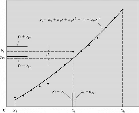
FIGURE 8.1

Least-squares regression analysis.

value calculated from the analytical expression and its corresponding mea-

sured y

value is a minimum (the diﬀerences are squared to avoid adding

compensating negative and positive diﬀerences). The best ﬁt would be ob-

tained by continually changing the coeﬃcients (a

through a

) in the an-

alytical expression until the diﬀerences are minimized. This, however, can

be quite tedious unless a formal approach is taken and some simplifying

assumptions are made.

Consider the data presented in Figure 8.1. The goal is to ﬁnd the values

of the a coeﬃcients in the analytical expression y

= a

+ a

x + a

... + a

that best ﬁts the data. To proceed formally, D is deﬁned as

the sum of the squares of all the vertical distances (the d

’s) between the

measured and calculated values of y (between y

and y

), as

D =

i=1

− y

)

i=1

− {a

+ a

+ ... + a

})

. (8.3)

Implicitly, it is assumed in this process that y

is normally distributed with a

true mean value of y

and a true variance of σ

. The independent variable x

is assumed to have no or negligible variance. Thus, x

= x

, where x

denotes

the true mean value of x. Essentially, the value of x is ﬁxed, known, and

with no variance, and the value of y is sampled from a normally distributed

population. Thus, all of the uncertainty results from the y value. If this

Regression and Correlation 299

were not the case, then the y

value corresponding to a particular y

value

would not be vertically above or below it. This is because the x

value

would fall within a range of values. Consequently, the distances would not

be vertical but rather at some angle with respect to the ordinate axis. Hence,

the regression analysis approach being developed would be invalid.

Now D is to be minimized. That is, the value of the sum of the squares

of the distances is to be the least of all possible values. This minimum is

found by setting the total derivative of D equal to zero. This actually is a

minimization of χ

(see [3]). Thus,

dD = 0 =

∂D

∂a

∂D

∂a

+ ... +

∂D

∂a

. (8.4)

For this equation to be satisﬁed, a set of m + 1 equations must be solved

for m + 1 unknowns. This set is

∂D

∂a

= 0 =

∂

∂a

i=1

∂D

∂a

= 0 =

∂

∂a

i=1

... , and

∂D

∂a

= 0 =

∂

∂a

i=1

. (8.5)

This set of equations leads to what are called the normal equations

(named by Carl Friedrich Gauss).

8.4 Linear Analysis

The simplest type of least-squares regression analysis that can be performed

is for the linear case. Assume that y is linearly related to x by the expression

= a

+ a

x. Proceeding along the same lines, for this case only two

equations (here m + 1 = 1 + 1 = 2) must be solved for two unknowns, a

and a

, subject to the constraint that D is minimized.

When dD = 0,

∂D

∂a

= 0 =

∂

∂a

i=1

− (a

+ a

)]

= −2

i=1

− a

). (8.6)

300 Measurement and Data Analysis for Engineering and Science

Carrying through the summations on the right side of Equation 8.6 yields

i=1

= a

N + a

i=1

. (8.7)

Also,

∂D

∂a

= 0 =

∂

∂a

i=1

− (a

+ a

)]

= −2

i=1

− a

). (8.8)

This gives

i=1

= a

i=1

+ a

i=1

. (8.9)

Thus, the two normal equations become Equations 8.7 and 8.9. These can

be rewritten as

¯y = a

+ a

¯x (8.10)

and

xy = a

¯x + a

. (8.11)

From the ﬁrst normal equation it can be deduced that a linear least-squares

regression analysis ﬁt will always pass through the point (¯x, ¯y). Equations

8.7 and 8.9 can be solved for a

and a

to yield

i=1

−

i=1

/∆, (8.12)

i=1

−

i=1

/∆, and (8.13)

∆ = N

i=1

−

i=1

. (8.14)

Linear regression analysis also can be used for a higher-order expres-

sion if the variables in expression can be transformed to yield a linear ex-

pression. This sometimes is referred to as curvilinear regression analysis.

Such variables are known as intrinsically linear variables. For this case,

a least-squares linear regression analysis is performed on the transformed

variables. Then the resulting regression coeﬃcients are transformed back to

yield the desired higher-order ﬁt expression. For example, if y = ax

, then

log

y = log

a + b log

x. So, the least-squares linear regression ﬁt of the

data pairs [log

x, log

y] will yield a line of intercept log

a and slope b.

Regression and Correlation 301

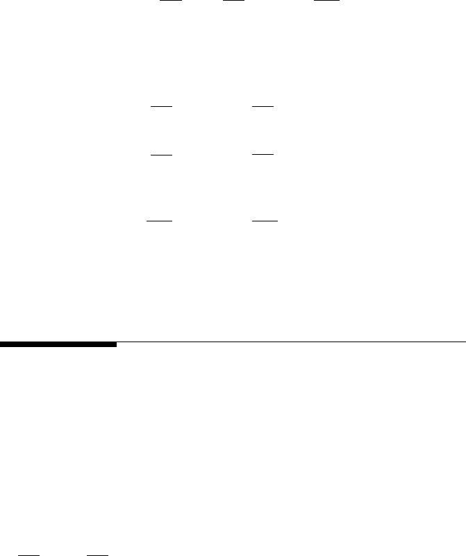
FIGURE 8.2

Regression ﬁt of the model y = ax

with data.

The resulting best-ﬁt values of a and b can be determined and then used in

the original expression.

Example Problem 8.1

Statement: An experiment is conducted to validate a physical model of the form

y = ax

. Five [x, y] pairs of data are acquired: [1.00, 2.80; 2.00, 12.5; 3.00, 25.2; 4.00,

47.0; 5.00 73.0]. Find the regression coeﬃcients a and b using a linear least-squares

regression analysis.

Solution: First express the data in the form of [log

x, log

y] pairs. This yields

the transformed data pairs [0.000, 0.447; 0.301, 1.10; 0.477, 1.40; 0.602, 1.67; 0.699,

1.86]. A linear regression analysis of the transformed data yields the best-ﬁt expression:

log

y = 0.461 + 2.01 log

x. This implies that a = 2.89 and b = 2.01. Thus, the best-

ﬁt expression for the data in its original form is y = 2.89x

2.01

. This best-ﬁt expression

is compared with the original data in Figure 8.2.

A similar approach can be taken when using a linear least-squares regres-

sion analysis to ﬁt the equation E

= A + B

√

U, which is King’s law. This

law relates the voltage, E, of a constant-temperature anemometer to a ﬂuid’s

velocity, U. A regression analysis performed on the data pairs [E

√

U] will

yield the best-ﬁt values for A and B. This is considered in homework prob-

lem 7.

302 Measurement and Data Analysis for Engineering and Science

8.5 Regression Parameters

There are several statistical parameters that can be calculated from a set of

data and its best-ﬁt relation. Each of these parameters quantiﬁes a diﬀerent

relationship between the quantities found from the data (the individual

values x

and y

and the mean values

x and

y) and from its best-ﬁt relation

(the calculated values).

Those quantities that are calculated directly from the data include the

sum of the squares of x, S

, the sum of the squares of y, S

, and the sum

of the product of x and y, S

. Their expressions are

≡

i=1

−

i=1

− N

, (8.15)

≡

i=1

−

i=1

− N

, (8.16)

and

≡

i=1

−

x)(y

−

y) =

i=1

− N

y. (8.17)

All three of these quantities can be viewed as measures of the square of the

diﬀerences or product of the diﬀerences between the x

and y

values and

their corresponding mean values. Equations 8.15 and 8.17 can be used with

the normal equations of a linear least-squares regression analysis to simplify

the expressions for the linear case’s best-ﬁt slope and intercept, where

b = S

(8.18)

and

a = ¯y − b¯x. (8.19)

Those quantities calculated from the data and the regression ﬁt include

the sum of the squares of the regression, SSR, the sum of the squares of

the error, SSE, and the sum of the squares of the total error, SST . Their

expressions are

SSR ≡

i=1

−

, (8.20)

SSE ≡

i=1

− y

)

, (8.21)

and

Regression and Correlation 303

SST ≡ SSE + SSR =

i=1

− y

)

i=1

−

. (8.22)

All three of these can be viewed as quantitative measures of the square of the

diﬀerences between the ¯y and y

values and their corresponding y

values.

SSR is also known as the explained variation and SSE as the unexplained

variation. Their sum, SST, is called the total variation. SSR is a measure of

the amount of variability in y

accounted for by the regression line and SSE

of the remaining amount of variation not explained by the regression line.

It can be shown further (see [5]) that

SST =

i=1

−

= S

. (8.23)

The combination of Equations 8.22 and 8.23 yields what is known as the

sum of squares partition [5] or the analysis of variance identity [6]

i=1

−

i=1

− y

)

i=1

−

. (8.24)

This expresses the three quantities of interest (y

, y

, and

y) in one equation.

An additional and frequently used parameter that characterizes the qual-

ity of the best-ﬁt is the standard error of the ﬁt, S

≡

SSE

N − 2

i=1

− y

)

N − 2

. (8.25)

This is equivalent to the standard deviation of the measured y

values with

respect to their calculated y

values, where ν = N − (m + 1) = N − 2 for

m = 1.

Example Problem 8.2

Statement: For the set of [x,y] data pairs [0.5, 0.6; 1.5, 1.6; 2.5, 2.3; 3.5, 3.7; 4.5,

4.2; 5.5, 5.4], determine ¯x, ¯y, S

, S

, and S

. Then determine the intercept and the

slope of the regression line using Equations 8.18 and 8.19 and compare the values to

those found by performing a linear least-squares regression analysis. Next, using the

regression ﬁt equation determine the values of y

. Finally, calculate SSE, SSR, and

SST . Show, using the results of these calculations, that SST = SSR + SSE.

Solution: Direct calculations yield ¯x = 3.00, ¯y = 2.97, S

= 17.50, S

= 15.89,

and S

= 16.60. The intercept and the slope values are a = 0.1210 and b = 0.9486

from Equations 8.19 and 8.18, respectively. The same values are found from regression

analysis. Thus, from the equation y

= 0.1210 + 0.9486x

the y

values are 0.5952,

1.5438, 2.4924, 3.4410, 4.3895, and 5.3381. Direct calculations then give SSE = 0.1470,

SSR = 15.7463, and SST = 15.8933. This shows that SSR + SSE = 15.7463 + 0.1470

= 15.8933 = SST , which follows from Equation 8.24.

304 Measurement and Data Analysis for Engineering and Science

Historically, regression originally was called reversion. Reversion referred

to the tendency of a variable to revert to the average of the population from

which it came. It was Francis Galton who ﬁrst elucidated the property of

reversion ([14]) by demonstrating how certain characteristics of a progeny

revert to the population average more than to the parents. So, in general

terms, regression analysis relates variables to their mean quantities.

8.6 Conﬁdence Intervals

Thus far it has been shown how measurement uncertainties and those intro-

duced by assuming an incorrect order of the ﬁt can contribute to diﬀerences

between the measured and calculated y values. There are additional uncer-

tainties that must be considered. These arise from the ﬁnite acquisition of

data in an experiment. The presence of these additional uncertainties af-

fects the conﬁdence associated with various estimates related to the ﬁt. For

example, in some situations, the inverse of the best-ﬁt relation established

through calibration is used to determine unknown values of the indepen-

dent variable and its associated uncertainty. A typical example would be to

determine the value and uncertainty of an unknown force from a voltage

measurement using an established voltage-versus-force calibration curve. To

arrive at such estimates, the sources of these additional uncertainties must

be examined ﬁrst.

For simplicity, focus on the situation where the correct order of the ﬁt is

assumed and there is no measurement error in x. Here, σ

= σ

. That is,

the uncertainty in determining a value of y from the regression ﬁt is solely

due to the measurement error in y.

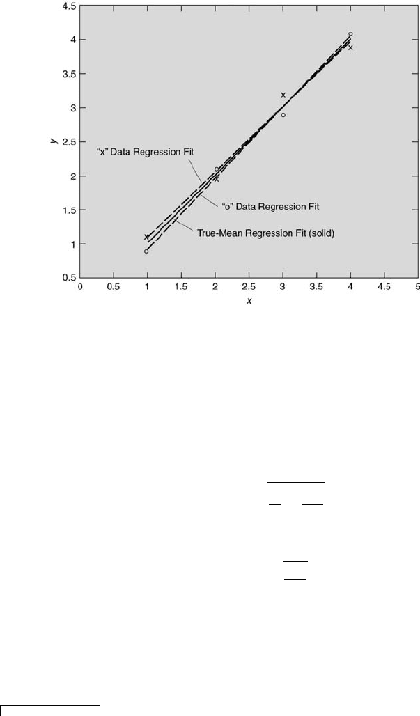
Consider the following situation, as illustrated in Figure 8.3, in which

best ﬁts for two sets of data obtained under the same experimental condi-

tions are plotted along with the data. Observe that diﬀerent values of y

are

obtained for the same value of x

each time the measurement is repeated

(in this case there are two values of y

for each x

). This is because y is a

random variable drawn from a normally distributed population. Because x

is not a random variable, it is assumed to have no uncertainty. So, in all

likelihood, the best-ﬁt expression of the ﬁrst set of data, y = a

x, will be

diﬀerent from the second best-ﬁt expression, y = a

+ b

x, having diﬀerent

values for the intercepts (a

6= a

) and for the slopes (b

6= b

The true-mean regression line is given by Equation 8.45 in which x = x

The true intercept and true slope values are those of the underlying popu-

lation from which the ﬁnite samples are drawn. From another perspective,

the true-mean regression line would be that found from the least-squares

linear regression analysis of a very large set of data (N >> 1).

Regression and Correlation 305

FIGURE 8.3

Linear regression ﬁts for two ﬁnite samples and one very large sample.

Recognizing that such ﬁnite sampling uncertainties arise, how do they

aﬀect the estimates of the true intercept and true slope? The estimates for

the true intercept and true slope values can be written in terms of the above

expressions for S

and S

[5],[6]. The estimate of the true intercept of the

true-mean regression line is

α = a ± t

N−2,P

¯x

. (8.26)

The estimate of the true slope of the true-mean regression line is

β = b ± t

N−2,P

. (8.27)

As N becomes larger, the sizes of the conﬁdence intervals for the true in-

tercept and true slope estimates become smaller. The value of a approaches

that of α, and the value of b approaches that of β. This simply reﬂects

the former statement, that any regression line based upon several N will

approach the true-mean regression line as N becomes large.

Example Problem 8.3

Statement: For the set of [x,y] data pairs [1.0, 2.1; 2.0, 2.9; 3.0, 3.9; 4.0, 5.1; 5.0,

6.1] determine the linear best-ﬁt relation using the method of least-squares regression