Peube J-L. Fundamentals of fluid mechanics and transport phenomena
Подождите немного. Документ загружается.

General Properties of Flows 293
Integrating [6.57] between 0 and 1, we obtain:
01
1
0
2
³
KKM
W
M
d
m
k
[6.58]
Equation [6.58] allows us to determine the unknown
W
if the function
M
is known.
It remains to choose the function
K
M
, whose general shape we know in the phase
plane from the discussion of section 6.3.1.1. The simplest algebraic function
satisfying conditions [6.57] is:
2
1
KM
[6.59]
Substituting into [6.58] we obtain:
0
3
1
2
m
k
W
whose positive root
km
3 only is acceptable. Thus, for the period
kmT
34
we obtain the value
928.634
which is slightly larger than the exact value
26.28
ʌ
(error of 10%). The reader will note that the error level is quite small,
given the crudeness of the computation.
However, we can hope to improve the result relatively easily by imposing
supplementary conditions resulting from equation
[6.57] on the second derivative
K
M
at instants 0 and 1:
01,0
2
M
W
M
m
k
[6.60]
Consider firstly second conditions [6.60]:
01
M
. The simplest polynomial
satisfying this and conditions [6.55] is of third order:
22
3
1
32
KK
KM
[6.61]
Substituting into equation [6.58] gives:
0
4
5
3
2
m
k
W
294 Fundamentals of Fluid Mechanics and Transport Phenomena
We therefore obtain
kmT 51244
W
; the value 197.65124 only
differs from the exact value by 1.4%.
The simplest polynomial satisfying the conditions [6.55] and [6.60] is of fourth
order:
43
4322
21
36
5
2
KK
KKKW
KM
¸
¸
¹
·
¨
¨
©
§
m
k
hence:
2
6
1
2
m
k
W
M
and
10
7
40
2
1
0
³
m
k
d
W
KKM
As the form of the curve representing the function
M
depends on the unknown
parameter
mk
2
W
, we obtain, by substituting into [6.58] a second order equation:
02
15
13
40
1
2
2
2
¸
¸
¹
·
¨
¨
©
§
m
k
m
k
WW
which has roots 2.497 and 32.16. It is easy to see that the second value is not
suitable,
M
having to be positive on the interval [0,1]. With the first value, the
calculation of the period gives:
k
m
T
k
m
32.6458.1
WW
The use of boundary conditions taken from the equation for the second
derivative thus leads to an improvement (error less than 1%). It should be noted
however that it is not possible to further improve the results of such a method, which
only uses local data at the extremities of the interval considered.
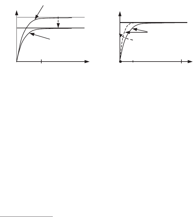
6.3.2.3. Damping of the oscillations
In an oscillatory regime, the essential movement corresponds to an exchange
between the kinetic and potential energy terms; only a small amount of the
mechanical energy is dissipated in each period. The interest of the kinetic energy
theorem [6.54] is that it gives an expression for the dissipated energy as a function
General Properties of Flows 295
of the variation of total mechanical energy: this is equal to the variation of maximum
kinetic energy
2
2
m
xm
, )(tx
m
being the maximum velocity value at each stretching
value of the mass m equal to zero. During a half-period 2
W
(notation as in the
preceding section) contained between two instants t and t + 2
W
where the elongation
is zero (
m
xx
), equation [6.54] translates this mechanical energy variation:
³
¸
¸
¹
·
¨
¨
©
§
W
W
W
G
2
2
12
12
2
2
2
1
2
t
t
p
p
dtxfxm
xm
[6.62]
Suppose as before that the amplitude of the velocity
m
x
varies only slightly and
that it can be considered as a constant during the half-period, while the velocity
variation is symmetric with respect to the instant
W
(Figure 6.11b). The law for the
velocity
K
M
0
x
t
x
results from the choice of the preceding function
K
M
:
00
with: 1
1
mm
! t
xt x! tx x x!
!
Taking the time origin at the beginning of the half-period, at the instant where
0 x
, and designating the velocity amplitude by
m
x
, gives, after substitution into
[6.62]:
³³
1
0
2
2
2
2
22
1
2
2
KKM
M
W
G
W
d
xf
dtxfx
m
m
t
t
m
[6.63]
Relation [6.63] is a finite difference equation with a step 2
W
for the amplitude
m
x
, which we can replace with the differential equation:
1
2
2
2
0
2
with:
2
1
m
m
!d
dx
m
fx
dt
!
¨
or:
0
m
m
x
dt
xd
f
m
D
[6.64]
296 Fundamentals of Fluid Mechanics and Transport Phenomena
The differential equation [6.64] can be solved as before using a global method.
We will here simply note that it represents a first order damped system with time
constant
fm
a
D
W
.
It remains to calculate the constant
D
. From the parabolic law of motion [6.59]
we have:
The third order law of motion [6.61] gives:
The exact solution for the damping is
f
m
a
2
W
. The error is a little greater than
for the calculation of the period: this is because a given approximation is always
better for a function
M
than for its derivative
M
.
6.4. Small parameters and perturbation phenomena
6.4.1. Introduction
The equations governing a physical phenomenon involve various non-
dimensional parameters. Very often, some of these are small. The associated terms
appear as a perturbation of the equations which are obtained when these terms are
zero. Mathematical phenomena associated with these perturbation terms can be
complex and their study should be carefully effected in order to understand their
precise role. We will limit ourselves in this section to the usual elementary cases in
fluid mechanics.
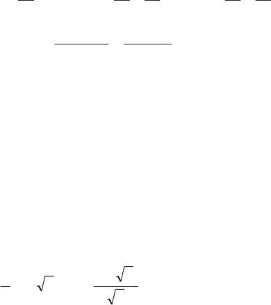
6.4.2. Regular perturbation
6.4.2.1.
Elementary example
A
perturbation
is called
regular
if the effects resulting from the perturbations
terms are everywhere in the same order of magnitude as the parameter which
characterizes them. A good example involves a first order damped system governed
by the following equation with the small parameter
H
:
General Properties of Flows 297
001
H xxx
whose solution is (Figure 6.12a):
)1(1
t
ex
H
.
This idea of a regular perturbation is associated with the mathematical idea of
uniform convergence which we will recall here briefly: a family of functions ),(
Htf
converges uniformly towards the function )0,(
tf
if the difference between the two
functions is independent of the value of t on a closed interval, and tends to zero with
H
. The limit
)0,(
tf
of the family of functions is thus continuous. This condition is
visibly satisfied for the preceding example.
1
O
x
t
1-exp(-t /
H
)
H
1
O
x
t
1-exp(-t)
H
(1+
H
)[1-exp(-t)]
1+
H
(b) (a)
Ho
1 1
Ho
Figure 6.12.
(a) Regular perturbation; (b) singular perturbation
6.4.2.2.
Regular perturbation of linear differential equations
Consider the linear differential problem which depends on the parameter
H
,
whose solution
H
,
tx
converges uniformly towards
0,
tx
when the small
parameter
H
tends to zero; we can often search for
H
,
tx
in the form of a power
series expansion of the parameter
H
, if this parameter has been suitably chosen:
......,
2
2
10
HHH H txtxtxtxtx
i
i
[6.65]
Substituting the preceding expression into the differential equation, we obtain a
series in increasing powers of
H
, the identification of whose coefficients in the two
sides provides
successive differential equations
. Let us first consider a simple
example of a linear differential equation in order to illustrate the computation
5
mechanism. Consider the differential equation representing the movement of a point
subjected to a weak repulsive force,
t
varying on [0,1]:
5
We assume that the domain of study corresponds to an time interval bounded a priori in
order to ensure uniform convergence.
298 Fundamentals of Fluid Mechanics and Transport Phenomena
1000
xxatxtx
H
[6.66]
Substituting development [6.65] into differential equation [6.66], we obtain the
successive differential equations:
..............
0000
..............
0000
0000
1000
1
2212
1101
000
pppp
xxtxtx
xxtxtx
xxtxtx
xxatx
The first differential equation is the non-perturbed equation which corresponds
to 0
H
; the successive differential equations only depend on the functions already
calculated, of lower rank in the development. The boundary conditions can be
carried back into the first equation, provided they do not contain the parameter H.
The solution of the preceding system can be calculated immediately from place
to place and we thus obtain a series development of the solution:
>@
........,
!12!12
....,
,
!5!6
,
!3!4
,
2
1212
56
2
34
1
2
0
p
t
p
t
ax
tt
ax
tt
axt
t
ax
pp
p
[6.67]
However, a development including many terms is not of much interest,
particularly if we consider the computational methods used by computers.
Furthermore, if the parameter Htakes on values which require many terms of the
development, the principal properties of the unperturbed equation are significantly
modified: in other words the unperturbed equation is no longer a sufficiently
representative model for the mathematical and physical properties of the solution for
these values of H.
For example, we easily recognize that [6.67] is the series development of the
solution which is here easy to calculate directly:
>@
H
H
H
H
tsh
tch
a
x 1
General Properties of Flows 299
When
H
is no longer small, the preceding series development is of limited
practical interest, despite an infinite radius of convergence, as the behavior of the
perturbed solution is too far from that of the unperturbed solution.
6.4.2.3.
Regular perturbation of non-linear differential equations
Consider a given first order differential equation:
axxtfx H 0,,
Calculating the development of the function
H
,,
x
t
f
in increasing powers of
the small parameter H becomes quickly complicated, and in general we are satisfied
by a limited development. We will here only outline the principle of the method and
the beginning of the calculation.
As before, we seek a solution of the form [6.65]:
......,
2
2
10
HHH H
t
x
t
x
t
x
t
x
t
x
i
i
We have:
>@
....0,,
2
0,,0,,
2
1
0,,
0,,0,,0,,
0..,,
2
0..,,0..,,
0,,
2
0,,0,,,,
3
0
2
1
01002
2
0100
10
2
2
2
102
2
10
2
HH
H
H
H
HHHHH
H
HH
HHH
H
HHH
HHH
»
»
¼
º
«
«
¬
ª
xtf
x
xtfxxtfxtfx
xtfxxtfxtf
xxtfxxxtfxxxtf
xtfxtfxtfxtf
xxxx
x
Substituting the preceding development into the differential equation and
identifying the following increasing powers of the small parameter H, we obtain:
000,,
2
0,,0,,
2
1
0,,
000,,0,,
000,,
20
2
1
010022
10011
000
xxtf
x
xtfxxtfxtfxx
xxtfxtfxx
axxtfx
xxxx
x
HHH
H
The first differential equation corresponds to the zero perturbation for H. We note
that the successive differential equations are linear for the corresponding unknown
function, with a right hand side which only depends on the previous solutions. The
300 Fundamentals of Fluid Mechanics and Transport Phenomena
equation linearity facilitates their numerical resolution. However, the expressions for
the differential equations can quickly become complex.
The interest of regular perturbation methods is particularly evident for problems
governed by partial differential equations, if particular solutions can be found which
have a simple mathematical structure (for example, one which approaches
differential equations), in which case the equations resulting from the application of
the regular perturbation method have a structure analogous to the initial solution.
We will see different examples of these methods applied to slightly unsteady flows,
to thermal systems which do not vary too quickly, and to the problems where inertia
terms due to geometric variations must be accounted for.
6.4.2.4.
Choice of a perturbation parameter
The perturbation parameter chosen for a study is of the utmost importance.
Suppose that a model leads to the following equation:
Axtbtxax
n
n
¸
¸
¹
·
¨
¨
©
§
¦
0,
HH
[6.68]
It is clearly possible to seek a solution in the form of a development of the
solution in powers of
H
0
1
(, ) () ()
i
i
i
xt% xt % xt
d
However, it is more interesting to take
¦
f
1i
i
i
a
HHD
as the perturbation
parameter and to seek a solution of the differential equation:
Axtbtxax 0,
0
H
H
D
in the form
0
1
(, ) () ().
i
i
i
xt xt xt
d
We find for the successive differential equations:
1
1
()=- () (0) 0
( )=- x (0) 0
i
ioi jij j
j
ioi i i
xaxt axt x
xaxtx

General Properties of Flows 301
The system obtained is far simpler for
i
x
~
than for x
i
. The preceding example is
apparently rudimentary. However, it translates the fact that the model has attributed
an important role to the parameter D, rather than to
H
which was chosen in order to
establish the model. It is clear that we can have a better development with the
parameter
D
than with
H
. This problem of parameter choice is often encountered in
order to best represent the range of solutions, for example, for solutions of boundary
layer equations ([SCH 99], [YIH 77]). The term b(t) of [6.68] can depend on
H
which must therefore express as a function of
D
.
The method can be applied to partial differential equations. We will later see
some examples of this (section 6.4.2.6). Suitable variable changes also allows the
modification or simplification of the differential problem (section 8.5.3.2).
The practical limits of the preceding method are determined by the convergence
of the entire series, but even more by the speed of convergence of the series
obtained. Methods for accelerating the convergence can be used here ([ABR 65]
p. 16, [BRE 91]).
6.4.2.5.
Regular perturbations and orders of magnitude
In the domain of studies where the orders of magnitude of the terms are fixed,
knowledge of a solution (exact or approximate) of an unperturbed problem allows
the calculation of correctional terms for the solutions in the neighborhood of the
base solution.
The successive differential equations obtained are linear equations which all
have the same linear operator, the right hand sides being known at each stage from
the preceding solutions. Numerical solution is thus simplified. The computation of
higher order terms of the solution by means of analytical developments, is generally
difficult in practice, on account of its complexity.
6.4.2.6.
Applications in fluid mechanics
With the exception of viscous stresses, taking account of other phenomena in
fluid mechanics, when these are relatively weak, very often leads to regular
perturbations: unsteady effects in established flow (in other words a flow which is
independent of its initial conditions), effects of compressibility in steady flow, weak
geometric changes, etc.
Consider the established flow of an incompressible fluid with constant viscosity
in a rectilinear pipe of arbitrary cross-section (Figure 6.13), and let us suppose that
we have a Poiseuille flow, with a driving pressure gradient
xp ww , parallel to the
velocity in the direction Ox, which is a given function of time; the velocity satisfies
the following equation (from [4.21]) and boundary conditions:
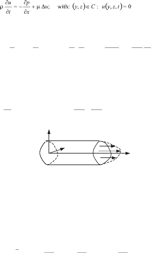
302 Fundamentals of Fluid Mechanics and Transport Phenomena
[6.69]
We will consider the following non-dimensional parameters and variables:
tf
x
p
U
D
T
D
D
z
D
y
zy
U
u
u
T
t
t
~
,
~
,
~~
~
22
w
w
¸
¸
¹
·
¨
¨
©
§
PP
U
H
where D and T are, respectively, a reference length for the cross-section and a unit of
time to be defined.
Equation [6.69] can be written:
¸
¸
¹
·
¨
¨
©
§
w
w
w
w
''
w
w
2
2
2
2
~
~
~
;
~
~
~
~
~
zy
utf
t
u
H
[6.70]
u
C
x
y
z
Figure 6.13.
Established flow in a cylindrical tube
Assume Hto be small and consider that equation [6.70] is the result of a regular
perturbation of this equation for
H
= 0. We seek the solution of [6.70] in the form
=0
=.
f
i
i
i
u İ u
Substituting into equation [6.70] and identifying terms following the
increasing powers of
H
, we obtain the system:
0
1
012 1
0 ; ; ; ...; ; ...
i
i
u
uu
ft u u u u
tt t
''' '
s
ss
ss s
with the boundary conditions:
~
~
,
~
0,
~
Czyzyu
i
0,1, 2,..., ,...in