Peube J-L. Fundamentals of fluid mechanics and transport phenomena

Подождите немного. Документ загружается.

General Properties of Flows 313

the instant t depends only on data from the past or the upstream region. This

explains the fact that the state of the matter in the cross-section depends on its

anterior state on the trajectory; the diffusion term of quantity G only provides a

limited action in this section, the suppression of the conduction term

ww

amounting to the suppression of all flux in the upstream direction.

The velocity components u and v are the unknowns of dynamic equation [6.76].

The demonstration of the parabolic character can be effected by introducing the

stream function

\

such that the mass conservation is satisfied:

xvyu ww ww

Equation [6.76] can thus be written:

222

xyxyytdt







\\\\\

[6.79]

In equation [6.79] the derivations with respect to x and t are of order 1, whereas

the derivation with respect to y is of order 3, which indicates the parabolic character

with respect to the variables x and t.

In applications, the hypotheses of section 6.5.1.1 are very often encountered.

Quasi-1D flows can be produced:

 when the geometric boundary conditions impose such an evolution: in flows in

pipes this kind of approximation exists for most macroscopic physical phenomena

(electric, electromagnetic, thermal, etc.);

 when diffusion phenomena in flows lead to weak fluxes of extensive quantities

in the axial direction Ox compared with the convection fluxes of these. In inviscid

fluids transport or propagation phenomena governed by the characteristics are, in

fact, perturbed by contact actions (viscosity, thermal conduction, diffusion, etc.), and

this leads to a transverse migration of the extensive quantities. The balance

equations contain high-order derivatives which “perturb” the convective transport

terms. In these situations, there exist non-dimensional parameters (Reynolds, Peclet

numbers, etc.) which take on high values.

We will successively examine two categories of problem in which the data are

different.

314 Fundamentals of Fluid Mechanics and Transport Phenomena

6.5.2. Flows in pipes

6.5.2.1. Nature of the problem

A pipe is a stream tube 6 materialized by a wall. The dominant velocity

component u in a cross-section is directed along its axis. The definition of the

problem to solve can be obtained as usual by combining the local balance equations

(mass, axial momentum, energy, etc.) with the initial and usual boundary conditions

on the wall

u(x,t)

S(x)

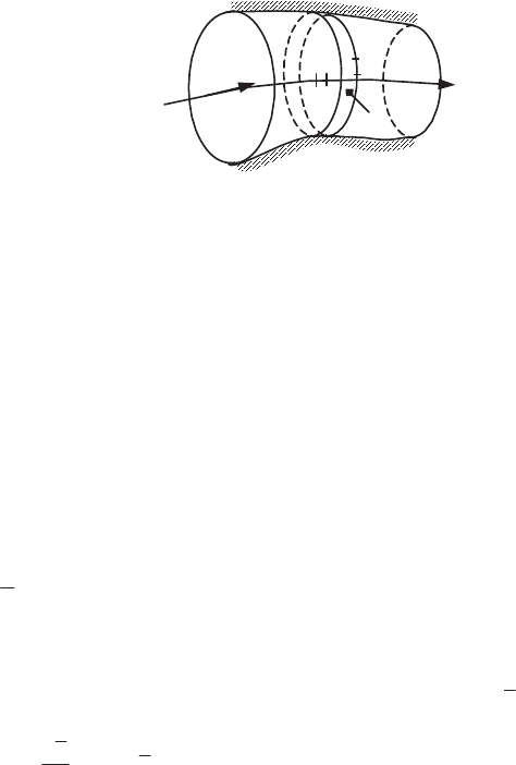
Figure 6.16.

Balance in a pipe

The geometric elements of the pipe are given, such that integration of the

dynamic equation leads to a relation between the volume (or mass) flow and a

pressure difference between two cross-sections. Calculation of the velocity

distribution (or of a quantity G) in a cross-section is an internal problem posed in

the interior domain of the stream tube 6 (Figure 6.16).

6.5.2.2.

Global balance equation for an extensive quantity in a pipe

The normal of a cross-section S(x) is here oriented parallel to Ox (orientation by

continuity). This convention requires a change in sign at the time of application of

Osstrogradski’s theorem to a closed surface 6 containing cross-sections. By

assumption, the lateral wall 6

is supposed impermeable to the flow, i.e.

dsnVg

. Consider the small domain

D of the pipe comprised between the

sections of abscissas x and x +

G

x of the lateral surface

G6

(Figure 6.16).

Formula [4.62] for the global balance of a volume quantity

g can be written:

dsnqdvdsnugdv

jGjGii

³³³³

¦6

 

[6.80]

General Properties of Flows 315

Taking account of the preceding assumptions, we have:

³³³³



6 S

dsxdvgudsdsnug

VGV

The density flux

is essentially normal to the lateral wall (section 6.5.1.2) for

irreversible changes (viscosity, conduction, diffusion) and the integral

dsnq

equal to

dqx

taken over the contour

of the cross-section (

is the flux

density of

, normal to the wall).

Substituting these expressions into [6.80] and dividing by

G

gives:



dqdsdsgu

GwG

³³³³





[6.81]

In the place of the volume quantity

, let us take the massive quantity

;

we obtain:



³³³³



GwG

dqdsugds

[6.82]

The quantity

³³

dsguugds

is the

flow of quantity

across the

cross-section

6.5.2.3.

Applications

Taking 1

, we have the

volume flow rate

udsq

across

Taking 1

, we have the equation for the

mass balance



[6.83]

with:

udsq

, the mass flow in the rate cross-section

The

momentum balance

along Ox can be obtained by applying formula [6.82] of

the quantity

. Supposing (section 6.5.1.3) that the driving pressure gradient

(here, the term

) is constant over the cross-section

, and designating by

the

viscous stress exerted by the fluid on the lateral wall

, we have:

316 Fundamentals of Fluid Mechanics and Transport Phenomena



Sdsu

³³³





[6.84]

Proceeding as before, kinetic energy equation [4.66] can immediately be written,

by noting that the power of the viscous forces on the external surface of

D is zero

because of the assumptions which have been made (zero velocity on the wall, and

quasi-1D approximation on

), we obtain:

Puds





³³

[6.85]

with:

)

dsP

, the power dissipated by viscosity per unit length of the pipe.

The first term of [6.85] gives the accumulation of kinetic energy in

transitional regime and the second expresses the flow rate of mechanical energy

across S.

The different forms of the

energy equation

seen in section 4.3.4 can be integrated

over the surface

(or in the domain

), but it is not possible to write down an

energy flow in the cross-section, except if we use initial formula [4.68] of the

balance equation which contains the flow of total enthalpy

=[ ( /2)]

ht m

* hV dq

across the section

Furthermore, the integral over

of the term





iij

can be transformed into a

surface integral, which is zero, as we have already said.

Proceeding as before for the thermal flux density, we obtain:

³³³³





TwT

dqdsuds

[6.86]

Recall that the power of an external force field is often negligible for a perfect

gas. The expressions for the internal specific energy

and the specific enthalpy

for

a perfect gas can be written:

;

1 



TCh

TCe

General Properties of Flows 317

The energy equation for an incompressible fluid of constant specific heat

(section 4.3.4.1.6 and equation [4.70]) can be written:



³³³³





TwTS

dqdsPuCTds

[6.87]

where, depending on the case, we used either C

or C

for the specific heat C.

6.5.2.4.

Average values of intensive quantities

As we have already said in section 1.4.2.5, to be consistent, the definition of

mean intensive values is effected such that the balance of the corresponding

extensive quantities is verified for the system studied. The application of this general

principle is expressed here by writing that values of the fluxes of extensive

quantities (mass, momentum, energy, etc.) in the cross-section

are identical either

by integration of local values or by using these mean values for balances. Then, we

take the following definitions:

 the mean density

 the mean velocity

dsu

 the mean temperature

(

= const):

dsuT

 and in general the mean quantity

dsug

These quantities are often called the

average mixing values

(or

mean mixing

values

), as they correspond to the intensive value represented by the variable

under

the assumption that the flow of

across the section

would directly fill a volume

where it should be mixed without any external input. The preceding definition of

supposes that the specific heat is independent of the temperature.

In cases where the same quantity contributes differently to several mean values,

we introduce a suitable coefficient, for example:

 the momentum coefficient

dsu

318 Fundamentals of Fluid Mechanics and Transport Phenomena

 the kinetic energy coefficient

dsu

These mean values and the preceding coefficients allow the equations for the

quasi-1D model of flow in a pipe to be written very simply in a form analogous to

the 1D slice approximation with uniform properties in the cross-section (see section

4.3.2.3.4). However, the system of differential equations obtained only determines a

solution if the preceding coefficients constitute data, which must be chosen more or

less empirically from assumptions derived from the velocity, temperature or

concentration profiles.

We will leave it to the reader to verify that in a laminar flow we have the

following values:

 uniform flow:

= 1;

 Poiseuille flow in a circular tube:

=2;

= 4/3.

In industrial pipe systems, the values of

and

are often of the order of 1.1 to

1.3 ([ASH 89], [IDE 99]). If the differences between the local velocity

and the

mean velocity

are small, the reader can verify that we have approximately



131  

The mechanical energy balance [6.85] (generalized Bernoulli’s theorem) in a

pipe for an incompressible fluid can be written with the definition of

vSv





[6.88]

We can thus define the

total mean driving pressure

ghpp

 .

The quantity

tmv

represents the

flow rate of mechanical energy across a

cross-section S

. Equation [6.88] becomes, on neglecting the power of the viscous

forces on 6 (approximation 2 of section 6.5.1.2):

Let

uuu



and neglect the term in

in the calculation of



General Properties of Flows 319





Integrating along the axis in the domain

included between two cross-sections

and

gives:



vtmtmv

Pppqdv

 

[6.89]

This equation is a model which reveals the inflows and outflows for the studied

domain of the pipe; it is particularly useful in steady flows for evaluating the

mechanical energy dissipated, using measurements of velocity distributions in the

sections

and

[IDE 99].

6.5.2.5.

Local equations

The local equations in the cross-section S of the stream tube are identical to the

local equations of the boundary layer which are developed in the following section.

6.5.3. The boundary layer in steady flow

6.5.3.1.

Introduction

We will limit our discussion in this section to the case of a steady flow of an

incompressible fluid of constant viscosity. The Navier-Stokes equations ([4.74] and

[4.75]) can be written with non-dimensional variables (section 4.6.1.3),

being

here the non-dimensional driving pressure:



3,2,1,;0

;

'



Rex

[6.90]

Under the usual conditions, the Reynolds number is very large compared to 1,

and the term

is weighted by a coefficient which is very small compared to 1.

This therefore appears to be a perturbation quantity whose nature we will study

using the procedure outlined in section 6.4.

320 Fundamentals of Fluid Mechanics and Transport Phenomena

6.5.3.2.

External solutions and the Euler equations

Assuming that the solution of the preceding equations and its derivatives vary at

the scale of 1, all the non-dimensional derivatives are in the order of 1, and the term

' is therefore very small compared to 1.

The dynamic equations can be reduced to the Euler equations:

)3,2,1,(



These are one order less, and require weaker boundary conditions than the

Navier-Stokes equations. It is clear from a physical point of view that we must

abandon the adherence condition, since the viscosity no longer exists, and the fluid

can therefore slide over the walls. We thus find ourselves in the singular

perturbation situation described in section 6.4.3.

6.5.3.3.

Finding a singular perturbation zone

Following the preceding reasoning, this zone cannot concern a zone of scale 1 in

all three dimensions. At least one of the dimensions of this zone must be small in

order for the value of a derivative to be sufficiently large to compensate the

coefficient 1/

. Where can such a zone be found? We note firstly that on account of

the transport of fluid and its properties, it is difficult for such a zone to

spontaneously appear in the heart of the flow. An exterior intervention is then

necessary in order to create a viscous phenomenon sufficiently large which then

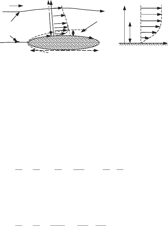
develops. This can only happen when the flow of an inviscid fluid encounters an

obstacle on the singular streamline which contains the stagnation point A of zero

velocity (Figure 6.17).

The subsequent velocity evolution on the wall streamlines of the inviscid fluid

lead to a non-zero sliding velocity which increases downstream of the point A. It is

then in the neighborhood of the wall that the viscosity must necessarily act.

The length of this zone is in the order of obstacle dimension

and its thickness

 is necessarily o

(L)

, otherwise we are back in the preceding situation. We must

therefore study a thin zone in the vicinity of the walls where we can make the

approximation of a quasi-1D flow. We will here consider a plane 2D flow over an

obstacle placed in a flow of uniform velocity

(Figure 6.17), and we will allow the

radii of curvature of the walls to be large compared with the thickness

General Properties of Flows 321

6.5.3.4.

Boundary layer equations

Let us consider an obstacle inside a uniform flow of an inviscid fluid at speed

Let us take a locally Cartesian coordinate system (

) defined in the following way

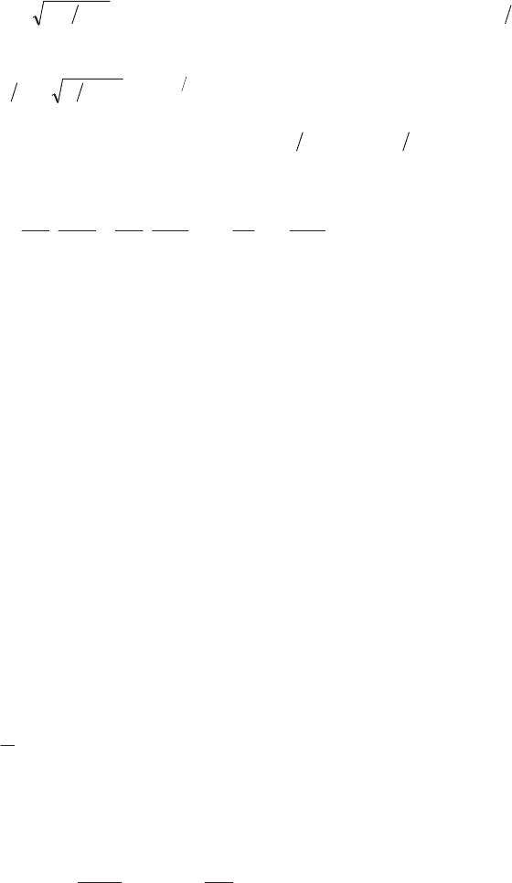
(Figure 6.17):

is the curvilinear abscissa evaluated algebraically on the wall

downstream of the stagnation point A on the obstacle, the coordinate

being

evaluated along the wall normal

. The velocity components are designated by (

u,v

)

in the coordinate system fixed to the wall and in its immediate vicinity.

G



flow of

inviscid flui

boundary layer

(x)

(b) (a)

G

Figure 6.17.

Boundary layer on the wall of an obstacle in uniform flow:

(a)

figure on the scale of

(b)

figure on the scale of



The discussion is as per section 6.5.1.3. The longitudinal velocity and

acceleration components are nearly parallel to the wall; the normal acceleration

component is negligible compared to the longitudinal component: the pressure,

constant across the thickness of the boundary layer is here only a function of the

abscissa x (section 6.5.1.3). However, in the dynamic equation, it is not possible to

neglect the

component in the material derivative which ensures a part of the

momentum transport (section 6.5.1.2). The dimensional equations of the 2D

boundary layer can thus be written:







[6.91]

The order of magnitude

of the boundary layer thickness can be obtained by

writing that the material derivative and the viscous stress term are of the same order

of magnitude (section 6.5.1.3):



322 Fundamentals of Fluid Mechanics and Transport Phenomena

where

UPG

, or by defining the Reynolds number

ULRe

with

the length



ULL

UPG

[6.92]

Introducing the stream function

(

xvyu

ww ww

; ), equations [6.91]

can be reduced to the equation:

xyxy





\\\\

[6.93]

The order of the derivatives with respect to

is less than the order of the

derivatives with respect to

in equation [6.93] which is parabolic: the

distribution of

the velocity at a given abscissa x

only depends on the upstream conditions of the

external velocity u

(x),

corresponding to values of

less than

6.5.3.5.

Boundary conditions

The boundary layer equations are clearly simpler than the Navier-Stokes

equations. We have already seen that the suppression of the transverse dynamic

equation leads to pressure being a function of the

direction only. We must now

express the adherence condition of the fluid at the wall, as this was our objective in

the introduction to the boundary layer.

 

00,0,0

xvxuy

We must now match the boundary layer and the external inviscid fluid flow. We

proceed in a first approximation as per section 6.4.3.3 by writing that the velocity at

the outer edge of the boundary layer is equal to the velocity



of the

inviscid

fluid on the wall in the absence of a boundary layer

 

xuyxu

ofo

[6.94]

The velocity



and

(

) satisfy Bernoulli’s theorem on the wall for an

inviscid fluid:



 

[6.95]

where

designates the static pressure in the external uniform flow of velocity