Samarskii A.A., Vabishchevich P.N. Numerical Methods for Solving Inverse Problems of Mathematical Physics

Подождите немного. Документ загружается.

396 Chapter 8 Other problems

measurements. In the case at hand, under the assumptions that the coefﬁcient k(u)

and the solution itself are smooth functions, it sufﬁces to additionally demand that the

function g(t) be a monotonic function. For deﬁniteness, we assume that

(t)>u

min

= 0, 0 < t < T, g(0) = 0, g (T ) = u

max

. (8.136)

In the inverse problem (8.132)–(8.135), we can pose a problem in which it is required

to ﬁnd the functional relation k(u) in the case of u

min

≤ u ≤ u

max

8.4.2 Functional optimization

In the approximate solution of the inverse problem (8.132)–(8.135), we can use the

variational formulation of this problem. We use the settings

K = L

min

, u

max

), (k, r )



max

min

k(u)r(u)du, k



(k, k)

In gradient iteration methods, we have to minimize the discrepancy functional that,

with regard to (8.135), looks as

J (k) =



m=1



(u(z

, t;k) − ϕ

(t))

dt (8.137)

under the conditions (8.132)–(8.134). In the Tikhonov regularization method, to be

regularized is the smoothing functional

(k) =



m=1



(u(z

, t;k) − ϕ

(t))

dt + αk

In using gradient iteration methods for the minimization of the functional J (k),we

have to calculate the gradient of the functional. Some difﬁculties arise owing to the

fact that the functional here is not quadratic. The gradient of J



(k) referring to the

increment δk is given by

δ J (k) = ( J



(k), δk)

+ s,

where δ J (k) = J (k + δk) − J (k) is the functional increment and

|s|

δk

→ 0 for δk → 0.

As we saw previously, the gradient of the discrepancy functional can be expressed

through the solution of some conjugate initial-boundary value problem. The most

general approach to the formulation of this problem is related with the consideration of

a problem on conditional minimization of the discrepancy functional on the solutions

Section 8.4 Coefﬁcient inverse problem for the nonlinear parabolic equation 397

of the boundary value problem for the ground state as a problem on unconditional

minimization by introducing Lagrange multipliers. As applied to the minimization

problem (8.137) under constraints (8.132)–(8.134), the Lagrange functional has the

form

G(k) = J (k) +





∂u

∂t

−

∂

∂x



k(u)

∂u

∂x



dx dt, (8.138)

where ψ(x, t ) is the Lagrange multipliers.

Let δG be the increment of the functional G corresponding to the increment δk and

δG = δ J + δ Q. (8.139)

We denote as δu the increment of u; then, we have for δ J :

δ J = 2



m=1



δu(u − ϕ

)δ(x − z

) dx dt, (8.140)

where δ(x) is the δ-function. Neglecting the second-order terms in (8.139), for the

second term in this formula we obtain

δQ =





∂δu

∂t

−

∂

∂x



k(u)

∂δu

∂x



−

∂

∂x



δk

∂u

∂x



dx dt. (8.141)

For the solution increments, from (8.133) and (8.134) we obtain:

δu(0, t) = 0,δu(l, t) = 0, 0 < t ≤ T,

δu(x, 0) = 0, 0 ≤ x ≤ l.

Hence, we have



∂δu

∂t

dx dt =−



δu

∂ψ

∂t

dx dt,

provided that

ψ(0, T ) = 0, 0 ≤ x ≤ l. (8.142)

In a similar manner, on setting the boundary conditions for ψ(x, t) in the form

ψ(0, t) = 0,ψ(l, t) = 0, 0 < t ≤ T (8.143)

we arrive at the equality



∂

∂x



k(u)

∂δu

∂x



dx dt =



δu

∂

∂x



k(u)

∂ψ

∂x



dx dt.

Besides, in the case of boundary conditions (8.143) we have



∂

∂x



δk

∂u

∂x



dx dt =−



δk

∂u

∂x

∂ψ

∂x

dx dt.

398 Chapter 8 Other problems

Now, we can rewrite expression (8.141) in the form

δQ =



δu



−

∂ψ

∂t

−

∂

∂x



k(u)

∂ψ

∂x



dx dt



δk

∂u

∂x

∂ψ

∂x

dx dt. (8.144)

With (8.140) and (8.144), we determine the function ψ(x, t) as the solution of the

equation

−

∂ψ

∂t

−

∂

∂x



k(u)

∂ψ

∂x



+ 2



m=1

(u − ϕ

)δ(x − z

) = 0,

0 < x < l, 0 ≤ t < T .

(8.145)

Thus, for the conjugate state to be found, we have to solve the well-posed initial-

boundary problem (8.142), (8.143), (8.145).

From (8.139) and (8.144), we obtain

δG =



δk

∂u

∂x

∂ψ

∂x

dx dt.

With regard to (8.138), this increment of the functional can be expressed in terms of



(k):

δG = (J



(k), δk)

In the calculation domain Q

we introduce new independent variables u(x, t) and

v(x, t), with the transformed Jacobian D(x, t)/D(u,v) = 0. With regard to our as-

sumptions (8.136) concerning the boundary condition (function g(t)), such a transform

is indeed possible. We therefore have:



δk

∂u

∂x

∂ψ

∂x

dx dt =



max

min

δk(u)



(u)

∂u

∂x

∂ψ

∂x

D(x , t)

D(u,v)

dv du

and, hence,



(k) =



(u)

∂u

∂x

∂ψ

∂x

D(x , t)

D(u,v)

dv, u

min

≤ u ≤ u

max

. (8.146)

The obtained representation (8.146) is not convenient for use in the development

of practical iteration solution methods for the coefﬁcient inverse problem (8.132)–

(8.135) because, in this case, we have a rather complex computational procedure for

the gradient of the discrepancy functional.

Section 8.4 Coefﬁcient inverse problem for the nonlinear parabolic equation 399

8.4.3 Parametric optimization

In the approximate solution of coefﬁcient inverse problems, special attention should be

paid to parametric identiﬁcation methods. In the gradient methods discussed above the

approximate solution is sought as a function of a continuous (or discrete, in the case

of difference approximation) argument. That is why here we use the term “functional

optimization”. Yet, another approach is possible, which can be considered as the pro-

jection method for solving inverse problems. In this method, the approximate solution

is represented in parametric form, and what is required is to ﬁnd the parameters in this

representation.

In a function space K , we choose a ﬁnite-difference subspace K

with some basis

(u), β = 1, 2,...,p. In the approximate solution of the coefﬁcient inverse problem

(8.132)–(8.135), the coefﬁcient to be found is represented in the form

(u) =



β=1

(u). (8.147)

In solving the inverse problem, the unknown coefﬁcients a

, β = 1, 2,..., p are to be

found.

The parametric identiﬁcation algorithm can be realized in two variants. We assume

that the accuracy in setting the input information is deﬁned by some quantity δ. Next,

we assume that in the model problem (8.132)–(8.135)

u(z

, t) = ϕ

(t), 0 < t ≤ T, m = 1, 2,...,M, (8.148)



m=1



(ϕ

(t) − ϕ

(t))

dt ≤ MTδ

. (8.149)

In solving the coefﬁcient problem (8.132)–(8.134), (8.148), (8.149), the ﬁrst vari-

ant of the parametric identiﬁcation algorithm is related with using a sufﬁciently high

dimensionality p of K

, in which case the inaccuracy in the approximation of k(u)

with the function k

(u) results in much lower solution inaccuracies at observation

points compared to initial inaccuracies (see (8.149)). In other words, the inaccura-

cies in (8.147) can be ignored in solving the inverse problem. Similar situation takes

place in difference discretization of the inverse problem: here, with sufﬁciently ﬁne

calculation grids used, we neglect the inaccuracies generated by the discretization.

Like with functional identiﬁcation, in the case under consideration the approximate

solution (8.147) can be regularized by minimizing the Tikhonov smoothing functional

for the vector a ={a

, a

,...,a

(a) =



m=1



(u(z

, t;a) − ϕ

(t))

dt + α



β=1

(8.150)

400 Chapter 8 Other problems

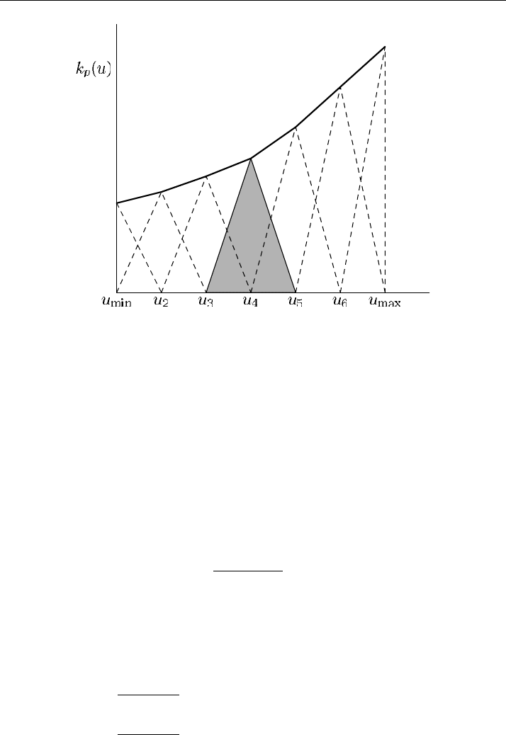
Figure 8.20 Piecewise-linear approximation

provided that the value of the regularization parameter α is properly matched with the

input-data inaccuracy (i.e., with the value of δ in (8.149)). An alternative here is an

iteration method for determining the vector a.

In the second variant of the parametric identiﬁcation algorithm, speciﬁc features of

parametric identiﬁcation are taken into account more fully. Here, the dimensionality

of K

, or the number of elements in the expansion (8.147), is used as the regulariza-

tion parameter. Here, we can speak of self-regularizing properties exhibited by the

discretization algorithm (8.147).

As a typical example of (8.147), consider piecewise linear approximation. We as-

sume that a grid

= u

min

+ (β − 1)

max

− u

min

p − 1

,β= 1, 2,...,p.

is introduced, uniform over the variable u. In this case (see Figure 8.20), the piecewise

linear ﬁnite functions η

(u), β = 1, 2,..., p are given in the form

(u) =

⎧

⎪

⎨

⎪

⎩

0, u < u

β−1

u − u

β−1

− u

β−1

, u

β−1

< u < u

β+1

− u

β+1

− u

, u

β−1

< u < u

0, u > u

β+1

β = 2, 3,...,p − 1,

and the coefﬁcients are a

= k

), β = 1, 2,...,p. In this representation of the

Section 8.4 Coefﬁcient inverse problem for the nonlinear parabolic equation 401

approximate solution, the mesh size over u or the total number p of nodes can be used

as a regularization parameter.

In the use of the regularization method (8.150), the computational algorithms for

parametric identiﬁcation (8.147) are related with the minimization problem for the

function p of the variable J

(a). Let us formulate a necessary condition for a

minimum that can be used to construct numerical algorithms for the parameters a

β = 1, 2,...,p. Immediately from (8.150), we have:

∂ J

∂a

= 2



m=1



(u(z

, t;a) − ϕ

(t))

∂u

∂a

dt + 2αa

. (8.151)

Relations (8.132)–(8.134) and representation (8.147) for ∂u/∂a

yield the following

boundary value problem:

∂v

∂t

−

∂

∂x



k(u)

∂v

∂x



∂

∂x



(u)

∂u

∂x



, 0 < x < l, 0 < t ≤ T , (8.152)

v(0, t) = 0,v(l, t) = 0, 0 < t ≤ T, (8.153)

v(x, 0) = 0, 0 ≤ x ≤ l. (8.154)

To obtain a more convenient representation for the ﬁrst term in the right-hand side

of (8.151), we formulate a boundary value problem for the conjugate state. Let the

function ψ(x, t) with some known u(x, t) be the solution of the boundary value prob-

lem (8.142), (8.143), (8.145). We multiply equation (8.152) through by ψ(x, t); then,

integrating the resulting equation over x and t, by direct calculations we obtain the

desired system of equations:



(u)

∂u

∂x

∂ψ

∂x

dx dt + 2αa

= 0,β= 1, 2,..., p. (8.155)

Around (8.155), we can construct the computational algorithms. In particular, we can

use iteration methods for determining the parameters a

, β = 1, 2,...,p. Here, the

complication owing to the nonlinear dependence of the ground state u(x, t) on the

sought coefﬁcient k(u) = k

(u) must be taken into account.

Under monotonic conditions for the boundary conditions of type (8.136), successive

identiﬁcation algorithms can be constructed. A similar local regularization procedure

was discussed above, in the consideration of evolutionary inverse problems in which

it was required to reconstruct the initial condition and the boundary conditions. In

the case of (8.132)–(8.136), at each time in the interval t ≤ t

∗

< T we can ﬁnd

the relation k(u) for u ≤ g(t

∗

). Such speciﬁc features of the coefﬁcient problem

under consideration can most easily be taken into account in the case of parametric

optimization of (8.147) in the class of piecewise constant functions. In the latter case

(see also Figure 8.21), with the use of the uniform grid

= u

min

+ β

max

− u

min

,β= 0, 1,...,p

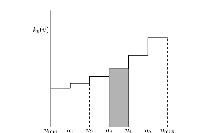
402 Chapter 8 Other problems

Figure 8.21 Piecewise-constant approximation

the trial functions are given in the form

(u) =

⎧

⎨

⎩

0, u < u

β−1

1, u

β−1

≤ u ≤ u

0, u > u

β = 1, 2,...,p. (8.156)

In the case of the latter parameterization, with u

β−1

≤ u ≤ u

it is required to ﬁnd just

one numerical parameter a

since the parameters a

, ν = 1, 2,...,β − 1 were found

previously. Such a procedure is possible not only with piecewise constant completion

of the unknown coefﬁcient, but also in using other approximations of (8.147), for

instance, with the piecewise linear approximation (see Figure 8.20).

8.4.4 Difference problem

Consider problems that arise when the parametric optimization algorithm in the vari-

ant of local regularization is used in the approximate solution of the coefﬁcient inverse

problem (8.132)–(8.135). Under the assumptions of (8.136), we solve the identiﬁca-

tion problem for the coefﬁcient k(u) in the class (8.147), (8.156).

We begin with constructing the difference analogue to the direct problem (8.132)–

(8.134). Over time, we introduce the simplest uniform grid

¯ω

= ω

∪{T }={t

= nτ, n = 0, 1,...,N

,τN

= T }

with some step size τ>0. To ﬁnd the approximate solution by the time t = t

,we

use the notations y

(x) = y(x, t

Section 8.4 Coefﬁcient inverse problem for the nonlinear parabolic equation 403

We complement the time-uniform grid with a grid non-uniform over u. With

(8.133), (8.136), we deﬁne

= g(t

), n = 0, 1,...,N

min

= g

< g

< ···< g

n−1

< g

< ···< g

= u

max

Using these data, one can construct a cruder grid over u:

= u

β−1

+ N

(β)

τ,

= u

min

, u

= u

max

,β= 1, 2,...,p.

(8.157)

In this way, between the nodes u

β−1

and u

we make N

(β)

time steps.

We denote as ¯ω a uniform grid with a step size h over the interval

 = [0, l]:

¯ω ={x | x = x

= ih, i = 0, 1,...,N, Nh = l}

Here, ω is the set of internal nodes, and ∂ω is the set of boundary nodes. We deﬁne

the difference operator

A(v)y =−(d(v)y

¯x

)

, x ∈ ω.

Then, we set the coefﬁcient d(v) in the form

d(v) = k(0.5(v(x) + v(x − h))), d(v) = 0.5(k(v(x − h)) + k(v(x))).

At the internal grid nodes over space, we put in correspondence to equation (8.132)

the purely implicit difference scheme

n+1

− y

+ A(y

n+1

= 0,

x ∈ ω, n = 0, 1,...,N

− 1.

(8.158)

The approximation of the boundary conditions (8.133) yields

n+1

(0) = 0, y

n+1

(l) = g

n+1

, n = 0, 1,...,N

− 1. (8.159)

To the initial condition (8.134), the following condition corresponds:

= 0, x ∈ ω. (8.160)

The matter of construction and computational realization of difference schemes for

the approximate solution of direct initially boundary problems of type (8.132)–(8.134)

was considered in more detail in Chapter 4. Of our primary concern here is the fol-

lowing question: how, based on the difference scheme (8.158)–(8.160), computational

algorithms for numerical solution of the coefﬁcient inverse problem (8.132)–(8.134)

can be constructed.

404 Chapter 8 Other problems

In using the piecewise constant approximation (8.147), (8.156), (8.157) of the un-

known coefﬁcient k(u), we can use the step-by-step identiﬁcation method. We assume

that some approximation for the nonlinear coefﬁcient is available for 0 ≤ u < u

β−1

The difference solution at the corresponding time, and at preceding times, is also

found. We seek the solution of the inverse problem for u

β−1

≤ u < u

We denote as L

(β)

the number of the time layer at which the solution u

is achieved.

With (8.157), we obtain:

(β)



γ =1

(γ )

, L

(0)

= 0,β= 1, 2,...,p.

In solving the inverse problem, the solution y

,0≤ l ≤ L

(β−1)

is known; according to

(8.147), (8.156), (8.157)), also known is the sought coefﬁcient k

in the same interval

(0 < u < u

β−1

Next, we solve the difference problem

n+1

− y

+ A(y

n+1

= 0, x ∈ ω,

n = L

(β−1)

+ 1, L

(β−1)

+ 2,...,L

(β)

(8.161)

n+1

(0) = 0, y

n+1

(l) = g

n+1

n = L

(β−1)

+ 1, L

(β−1)

+ 2,...,L

(β)

(8.162)

Here, only the coefﬁcient a

is unknown. To determine this coefﬁcient, we invoke

additional available information (see (8.148), (8.149)).

We assume that the observation points z

, m = 1, 2,...,M are some internal

nodes of the calculation grid over space. As the criterion for closeness of the ap-

proximate solution at these points to measured values, in solution of problem (8.161),

(8.162), in line with (8.148), it seems reasonable to use the criterion

(β)



m=1

(β)



n=L

(β−1)

) − ϕ

))

τ. (8.163)

In view of J

(β)

= J

(β)

), the parameter a

can be found from the minimum of the

function J

(β)

). In computational realization, to ﬁnd the minimum of (8.163), we

can use standard minimization methods for a function of one variable (the golden-

section method, the method of parabolas, etc.).

In the local regularization under consideration, matching with the input-data inac-

curacy can be achieved through a proper choice of the interval [u

β−1

, u

] (choice of

(β)

= L

(β)

−L

(β−1)

in (8.161), (8.162). Using the discrepancy principle and inequal-

ity (8.149), we choose a maximum N

(β)

for which

(β)

≤ MN

(β)

. (8.164)

Section 8.4 Coefﬁcient inverse problem for the nonlinear parabolic equation 405

In some critical cases, relation (8.164) can be violated at all N

(β)

; then, we have to

choose N

(β)

= 1.

8.4.5 Program

The computational algorithm for the successive determination of the nonlinear coefﬁ-

cient k(u) is realized in the program PROBLEM18. Consider some speciﬁc features of

this program.

The time interval is divided into equal subintervals; the total number of these subin-

tervals is p = 2

, ν = 0, 1,...,ν

max

(in the case of N

= 2

max

). The reﬁnement is

terminated on achievement of a certain level of discrepancy or on the condition that

subsequent densening of the grid does not decrease the discrepancy. To approximately

solve the nonlinear equation for the constant, we use the golden-section method.

Program PROBLEM18

C PROBLEM18 - COEFFICIENT INVERSE PROBLEM

C QUASI-LINEAR 1D PARABOLIC EQUATION

IMPLICIT REAL

8 ( A-H, O-Z )

PARAMETER ( DELTA = 0.02D0, N = 100, M = 128 )

DIMENSION X(N+1), Y(N+1), Y1(N+1), YT(N+1)

+ ,U(N+1,M+1), AKS(M+1), PHI(M+1), PHID(M+1)

+ ,BR(M+1), UL(M+1)

+ ,A(N+1), B(N+1), C(N+1), F(N+1)

+ ,ALPHA(N+2), BETA(N+2)

C PARAMETERS:

C XL, XR - LEFT AND RIGHT END POINTS OF THE GEGMENT;

C N + 1 - NUMBER OF NODAL POINTS OVER SPACE;

C M + 1 - NUMBER OF NODAL POINTS OVER TIME;

C XD - OBSERVATION POINT;

C PHI(M+1) - EXACT SOLUTION AT THE OBSERVATION POINT;

C PHID(M+1) - DISTURBED SOLUTION AT THE OBSERVATION POINT;

XL = 0.D0

XR = 1.D0

TMAX = 1.D0

XD = 0.6D0

EPSA = 1.D-4

EPSH = 1.D-4

OPEN (01, FILE=’RESULT.DAT’) ! FILE TO STORE THE CALCULATED DATA

C GRID

H =(XR-XL)/N

TAU = TMAX / M

DOI=1,N+1

X(I) = XL + (I-1)

END DO