Samarskii A.A., Vabishchevich P.N. Numerical Methods for Solving Inverse Problems of Mathematical Physics

Подождите немного. Документ загружается.

366 Chapter 8 Other problems

At the internal nodes, in using the purely implicit scheme we approximate equation

(8.54) with the difference equation

n+1

− y

− (ay

n+1

¯x

)

= 0, x ∈ ω, n = 0, 1,...,N

− 1, (8.79)

with, for instance, a(x) = k(x − 0.5h). The initial condition (8.56) yields:

(x) = 0, x ∈ ω. (8.80)

The second-kind boundary condition (8.55) is approximated on the solutions of

(8.54):

n+1

− y

−

n+1

− y

n+1

= 0, n = 0, 1,...,N

− 1. (8.81)

To the non-local boundary condition (8.57), we put in correspondence the non-local

difference condition

n+1

+ αy

n+1

= ϕ

n+1

, n = 0, 1,...,N

− 1. (8.82)

Realization of the difference scheme (8.79)–(8.82) implies solution of the three-

point difference problem at each time step with the non-local boundary conditions

(8.82). To this end, we can use some modiﬁcation of the standard sweep algorithm.

A second possibility was considered previously, in the discussion of non-local regu-

larization; this possibility is related with the use of some special representation of the

solution (see (8.63) and (8.72)).

We seek the solution of the difference problem (8.79)–(8.82) in the form

n+1

(x) = z

n+1

(x) + q(x)v

n+1

, x ∈¯ω. (8.83)

Here, similarly to (8.64)–(8.67), the mesh function z

(x) is deﬁned as the solution

of the following direct problem:

n+1

− y

− (az

n+1

¯x

)

= 0, x ∈ ω, n = 0, 1,...,N

− 1, (8.84)

(x) = 0, x ∈ ω, (8.85)

n+1

− y

−

n+1

− z

n+1

= 0, n = 0, 1,...,N

− 1, (8.86)

n+1

= 0, n = 0, 1,...,N

− 1. (8.87)

The mesh function q(x) (see (8.73), (8.74)) is deﬁned as the solution of the boundary

value problem

− (aq

¯x

)

= 0, x ∈ ω, (8.88)

Section 8.2 Non-local distribution of boundary conditions 367

−

− q

= 0, q

= 1. (8.89)

Substitution of (8.83) into (8.82) yields:

n+1

− z

n+1

α + q

, n = 0, 1,...,N

− 1. (8.90)

For the solution of the difference problem (8.79)–(8.82) to be found, we have to solve

two standard problems, problems (8.84)–(8.87) and (8.88), (8.89) and, then, ﬁnd the

function v

, n = 1, 2,...,N by formula (8.90); subsequently, the sought solution is

to be represented in the form (8.83).

8.2.5 Program

The above solution algorithm for the boundary value inverse problem (8.49), (8.50),

(8.52), (8.53) based on a non-local perturbation of the boundary condition is realized

in the program PROBLEM16.

Program PROBLEM16

C PROBLEM16 - IDENTIFICATION OF THE BOUNDARY CONDITION

C ONE-DIMENSIONAL NON-STATIONARY PROBLEM

C NON-LOCAL DISTURBANCE OF THE BOUNDARY CONDITION

IMPLICIT REAL

8 ( A-H, O-Z )

PARAMETER ( DELTA = 0.01D0,N=101,M=21)

DIMENSION X(N), Y(N), Z(N), Q(N)

+ ,FI(M), FID(M), FIY(M), U(M), UA(M)

+ ,A(N), B(N), C(N), F(N)

C PARAMETERS:

C XL, XR - LEFT AND RIGHT ENDS OF THE GEGMENT;

C N - NUMBER OF GRID NODES OVER SPACE;

C TMAX - MAXIMAL TIME;

C M - NUMBER OF GRID NODES OVER TIME;

C DELTA - INPUT-DATA INACCURACY LEVEL;

C FI(M) - EXACT DIFFERENCE BOUNDARY CONDITION;

C FID(M) - DISTURBED DIFFERENCE BOUNDARY CONDITION;

C U(M) - EXACT SOLUTION OF THE INVERSE PROBLEM

C (BOUNDARY CONDITION);

C UA(M) - APPROXIMATE SOLUTION OF THE INVERSE PROBLEM;

XL = 0.D0

XR = 1.D0

TMAX = 1.D0

OPEN ( 01, FILE=’RESULT.DAT’) ! FILE TO STORE THE CALCULATED DATA

C GRID

H=(XR-XL)/(N-1)

368 Chapter 8 Other problems

DOI=1,N

X(I) = XL + (I-1)

END DO

TAU = TMAX / (M-1)

C DIRECT PROBLEM

C BOUNDARY REGIME

DOK=1,M

T = (K-1)

TAU

U(K) = AF(T, TMAX)

END DO

C INITIAL CONDITION

T = 0.D0

DOI=1,N

Y(I) = 0.D0

END DO

C NEXT TIME LAYER

DOK=2,M

T=T+TAU

C DIFFERENCE-SCHEME COEFFICIENTS

C PURELY IMPLICIT SCHEME

DOI=2,N-1

A(I) = 1.D0 / (H

B(I) = 1.D0 / (H

C(I) = A(I) + B(I) + 1.D0 / TAU

F(I) = Y(I) / TAU

END DO

C BOUNDARY CONDITION AT THE LEFT AND RIGHT ENDS

B(1) = 2.D0 / (H

C(1) = B(1) + 1.D0 / TAU

F(1) = Y(1) / TAU

A(N) = 0.D0

C(N) = 1.D0

F(N) = U(K)

C SOLUTION OF THE PROBLEM ON THE NEXT TIME LAYER

ITASK = 1

CALL PROG3 ( N, A, C, B, F, Y, ITASK )

C SOLUTION AT THE LEFT BOUNDARY

FI(K) = Y(1)

FID(K) = FI(K)

END DO

C NOISE ADDITION TO THE SOLUTION OF THE BOUNDARY-VALUE PROBLEM

DOK=2,M

Section 8.2 Non-local distribution of boundary conditions 369

FID(K) = FI(K) + 2.D0

DELTA

(RAND(0)-0.5D0)

END DO

C INVERSE PROBLEM

C NON-LOCAL DISTURBANCE OF THE BOUNDARY CONDITION

C AUXILIARY MESH FUNCTION

C DIFFERENCE-SCHEME COEFFICIENTS

DOI=2,N-1

A(I) = 1.D0 / (H

B(I) = 1.D0 / (H

C(I) = A(I) + B(I) + 1.D0 / TAU

F(I) = 0.D0

END DO

C BOUNDARY CONDITION AT THE LEFT AND RIGHT END POINTS

B(1) = 2.D0 / (H

C(1) = B(1) + 1.D0 / TAU

F(1) = 0.D0

A(N) = 0.D0

C(N) = 1.D0

F(N) = 1.D0

C SOLUTION OF THE PROBLEM

ITASK = 1

CALL PROG3 ( N, A, C, B, F, Q, ITASK )

C ITERATIVE PROCESS FOR THE REGULARIZATION PARAMETER

IT=0

ITMAX = 100

ALPHA = 0.001D0

QQ = 0.75D0

100IT=IT+1

C INITIAL CONDITION

T = 0.D0

DOI=1,N

Y(I) = 0.D0

END DO

UA(1) = Y(N)

C NEXT TIME LAYER

DOK=2,M

T=T+TAU

C DIFFERENCE-SCHEME COEFFICIENTS

C PURELY IMPLICIT SCHEME

DOI=2,N-1

A(I) = 1.D0 / (H

B(I) = 1.D0 / (H

C(I) = A(I) + B(I) + 1.D0 / TAU

370 Chapter 8 Other problems

F(I) = Y(I) / TAU

END DO

C BOUNDARY CONDITION AT THE LEFT AND RIGHT END POINTS

B(1) = 2.D0 / (H

C(1) = B(1) + 1.D0 / TAU

F(1) = Y(1) / TAU

A(N) = 0.D0

C(N) = 1.D0

F(N) = 0.D0

C SOLUTION OF THE AUXILIARY PROBLEM ON THE NEXT TIME LAYER

ITASK = 1

CALL PROG3 ( N, A, C, B, F, Z, ITASK )

C SOLUTION AT THE RIGHT BOUNDARY

UA(K) = (FID(K) - Z(1)) / (ALPHA + Q(1))

C SOLUTION AT ALL NODES

DOI=1,N

Y(I) = Z(I) + Q(I)

UA(K)

END DO

C SOLUTION OF THE DIRECT PROBLEM WITH THE FOUND BOUNDARY CONDITION

C INITIAL CONDITION

T = 0.D0

DOI=1,N

Y(I) = 0.D0

END DO

FIY(1) = Y(1)

C NEXT TIME LAYER

DOK=2,M

T=T+TAU

C DIFFERENCE-SCHEME COEFFICIENTS

DOI=2,N-1

A(I) = 1.D0 / (H

B(I) = 1.D0 / (H

C(I) = A(I) + B(I) + 1.D0 / TAU

F(I) = Y(I) / TAU

END DO

C BOUNDARY CONDITION AT THE LEFT AND RIGHT END POINTS

B(1) = 2.D0 / (H

C(1) = B(1) + 1.D0 / TAU

F(1) = Y(1) / TAU

A(N) = 0.D0

C(N) = 1.D0

F(N) = UA(K)

Section 8.2 Non-local distribution of boundary conditions 371

C SOLUTION OF THE PROBLEM ON THE NEXT TIME LAYER

ITASK = 1

CALL PROG3 ( N, A, C, B, F, Y, ITASK )

FIY(K) = Y(1)

END DO

C CRITERION FOR THE EXIT FROM THE ITERATIVE PROCESS

SUM = 0.D0

DOK=1,M

SUM = SUM + (FIY(K) - FID(K))

TAU

END DO

SL2 = DSQRT(SUM)

IF (IT.GT.ITMAX) STOP

IF ( IT.EQ.1 ) THEN

IND=0

IF ( SL2.LT.DELTA ) THEN

IND=1

QQ = 1.D0/QQ

END IF

ALPHA = ALPHA

GO TO 100

ELSE

ALPHA = ALPHA

IF ( IND.EQ.0 .AND. SL2.GT.DELTA ) GO TO 100

IF ( IND.EQ.1 .AND. SL2.LT.DELTA ) GO TO 100

END IF

C RECORDING OF CALCULATED DATA

WRITE ( 01,

) (U(K), K = 1,M)

WRITE ( 01,

) (FID(K), K = 1,M)

WRITE ( 01,

) (UA(K), K = 1,M)

WRITE ( 01,

) (FIY(K), K = 1,M)

CLOSE ( 01 )

STOP

END

DOUBLE PRECISION FUNCTION AF ( T, TMAX )

IMPLICIT REAL

8 ( A-H, O-Z )

C BOUNDARY CONDITION AT THE RIGHT BOUNDARY

AF = 2.D0

T/TMAX

IF (T.GT.(0.5D0

TMAX)) AF = 2.D0

(TMAX-T)/TMAX

RETURN

END

The program implements the algorithm with non-locally perturbed boundary condi-

tions for problem (8.49), (8.50), (8.52), (8.53) with the coefﬁcient k(x) = const = 1

and with the non-local perturbation parameter chosen from the discrepancy.

372 Chapter 8 Other problems

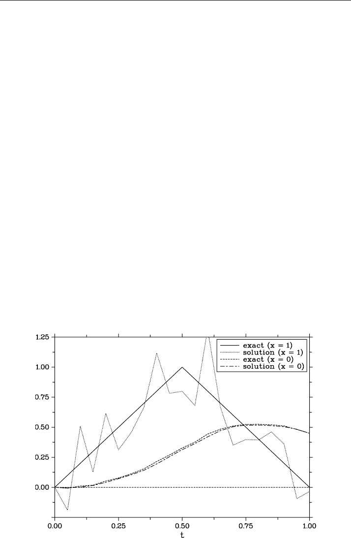
8.2.6 Computational experiments

The problem was solved using a uniform grid with h = 0.01 and τ = 0.05 in the

calculation domain with l = 1 and T = 1. The input data in the inverse problem were

taken from the solution of the direct problem with the right-end boundary condition

ψ(t) =



2t/T , 0 < t < T/2,

2(T − t)/T, T/2 < t < T.

The same model problem was considered above, when we discussed the algorithm

with continuation over the spatial variable.

The data calculated with the various input-data inaccuracy levels are shown in Fig-

ures 8.6–8.8. A comparison with the data obtained using the algorithm with contin-

uation over the spatial variable (see Figures 8.2, 8.4, 8.5) shows that the algorithm

with non-locally perturbed boundary condition is inferior in terms of data accuracy

because it poorly takes into account the speciﬁc features of the boundary value inverse

problems of interest. With this approach, we hardly can count on time ﬁltration of

high-frequency inaccuracies because here, in fact, we have regularization with respect

to the spatial variable.

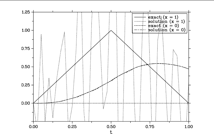
In many respects, the effect due to the regularization is provided at the expense of

cruder calculation grids along time (self-regularization effect). An illustration here

are the data calculated with a ﬁner grid along time (see Figure 8.9). The input-data

inaccuracies can be most distinctly identiﬁed by reducing the time step size. The latter

can be explicitly traced considering the formula for the solution at the right boundary,

since q

→ 0asτ → 0.

Figure 8.6 Inverse-problem solution obtained with δ = 0.01

Section 8.2 Non-local distribution of boundary conditions 373

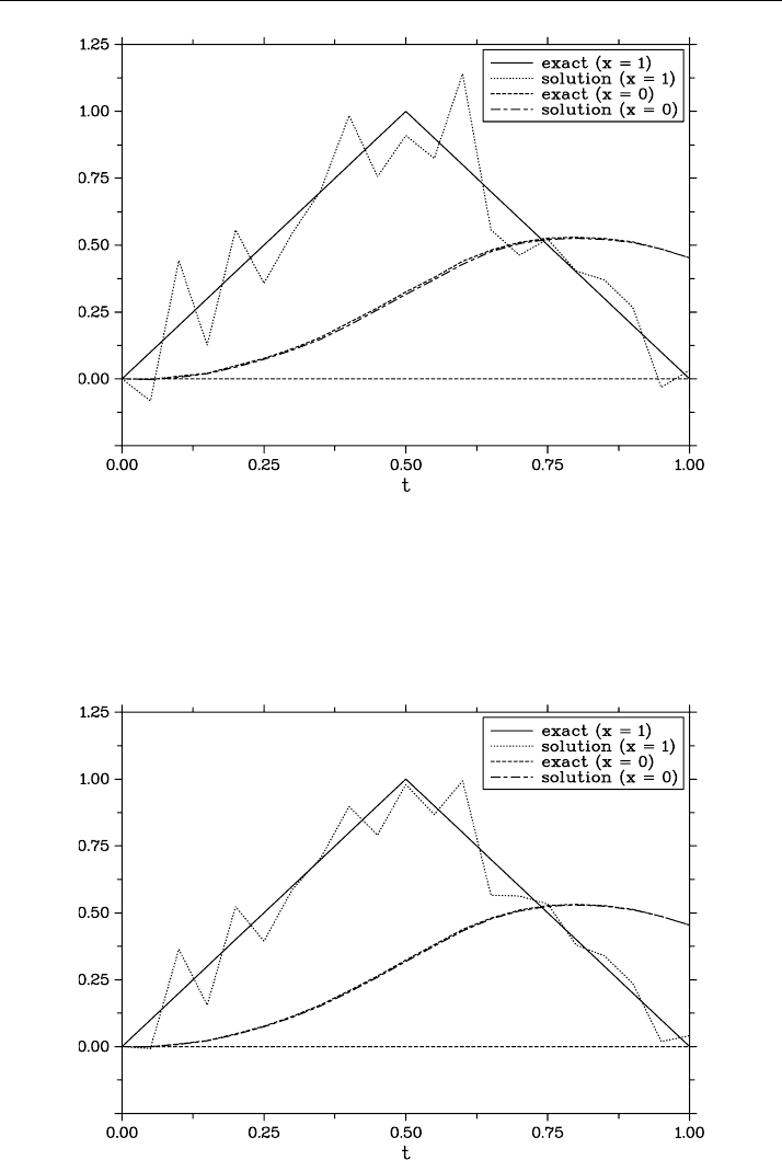
Figure 8.7 Inverse-problem solution obtained with δ = 0.005

Figure 8.8 Inverse-problem solution obtained with δ = 0.0025

374 Chapter 8 Other problems

Figure 8.9 Solutions obtained with δ = 0.0025 and τ = 0.025

8.3 Identiﬁcation of the boundary condition

in the two-dimensional problem

In this section, we consider the boundary-layer inverse problem for the two-

dimensional parabolic equation of second order. From data on some portion of the

boundary, it is required to reconstruct the boundary data on the other portion of the

boundary. To approximately solve the problem, we use the iteration method. Primary

attention is given to accurate formulation of the symmetrized operator equation of the

ﬁrst order at the differential and mesh levels.

8.3.1 Statement of the problem

To most powerful methods intended for the approximate solution of inverse problems

for mathematical physics equations, iteration methods belong. These methods rather

adequately take into account the general speciﬁc features of the problems. Very often,

the correct use of such methods is hampered by the necessity to perform certain analyt-

ical work primarily related with the fact that symmetrization of the corresponding op-

erator equation of the ﬁrst order is necessary. Similar problems are encountered in the

formulation of necessary minimum conditions in the Tikhonov regularization method

as applied to related optimum control problems for systems governed by mathematical

physics equations. Here, the matter of obtaining the symmetrized operator equation is

considered both on the differential level and on the mesh level.

Section 8.3 Identiﬁcation of the boundary condition in two-dimensional problems 375

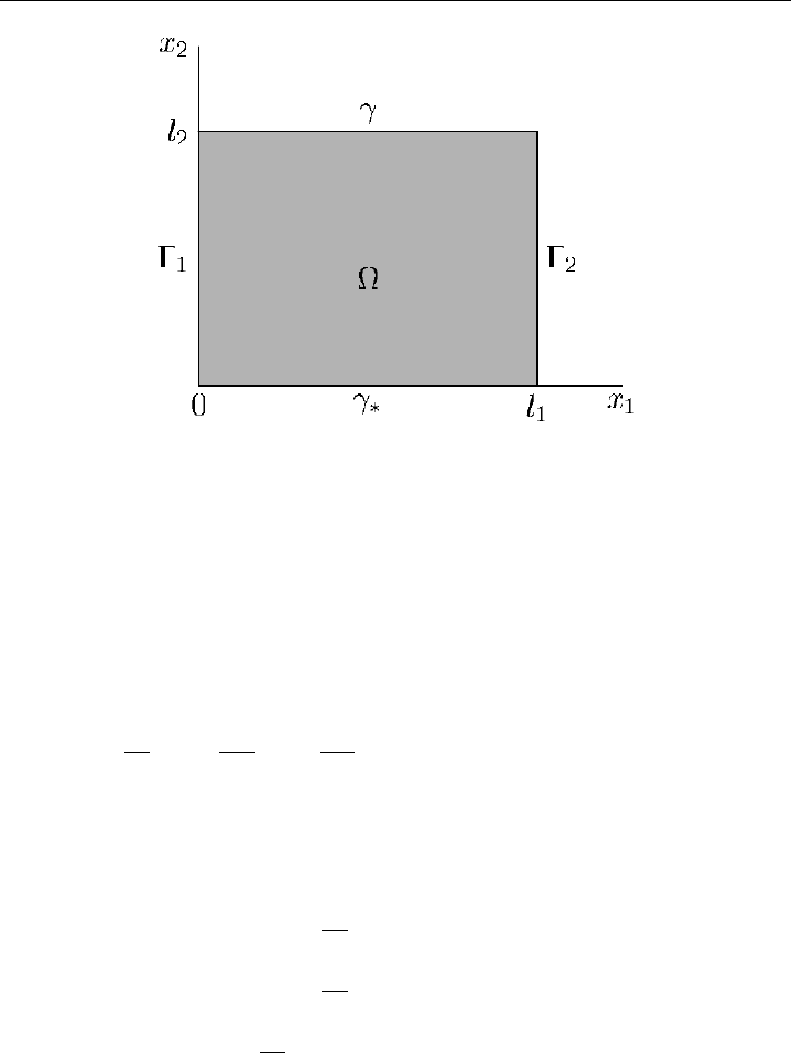
Figure 8.10 Calculation domain

As a model one, consider the two-dimensional problem in the rectangle

 ={x | x = (x

, x

), 0 < x

< l

,β= 1, 2}.

For the sides of , we use the following notations (see Figure 8.10):

∂ = γ

∗

∪ 

∪ γ ∪ 

,= 

∪ 

In , we seek the solution of the parabolic equation

∂u

∂t

−



β=1

∂

∂x



k(x)

∂u

∂x



= 0, x ∈ , 0 < t < T . (8.91)

We assume that k(x) ≥ κ, κ>0, x ∈ .

The starting point in the present consideration is the direct initial-boundary value

problem for equation (8.91), in which the boundary and initial conditions look as

k(x)

∂u

∂n

(x, t) = 0, x ∈ ∂γ

∗

, (8.92)

k(x)

∂u

∂n

(x, t) = 0, x ∈ , (8.93)

k(x)

∂u

∂n

(x, t) = μ(x

, t), x ∈ γ, (8.94)

u(x, 0) = 0, x ∈ . (8.95)

Consider an inverse problem in which it is required to identify the boundary condi-

tion on some portion of the boundary (on γ ). In the latter case, instead of (8.94) the

following condition is given:

u(x, t) = ϕ(x

, t), x ∈ γ

∗

. (8.96)