Samarskii A.A., Vabishchevich P.N. Numerical Methods for Solving Inverse Problems of Mathematical Physics

Подождите немного. Документ загружается.

356 Chapter 8 Other problems

B(I) = 1.D0 / (H

C(I) = A(I) + B(I) + 1.D0 / TAU

FF(I) = Y(I,K-1) / TAU

END DO

C BOUNDARY CONDITION AT THE LEFT AND RIGHT END POINTS

B(1) = 2.D0 / (H

C(1) = B(1) + 1.D0 / TAU

FF(1) = Y(1,K-1) / TAU

A(N) = 0.D0

C(N) = 1.D0

FF(N) = Q(K)

C SOLUTION OF THE PROBLEM ON THE NEXT TIME LAYER

ITASK = 1

CALL PROG3 ( N, A, C, B, FF, YY, ITASK )

DOI=1,N

Y(I,K) = YY(I)

END DO

C SOLUTION ON THE LEFT BOUNDARY

DOK=1,M

FI(K) = Y(1,K)

FID(K) = FI(K)

END DO

C NOISE ADDITION TO THE SOLUTION OF THE BOUNDARY-VALUE PROBLEM

DOK=2,M

FID(K) = FI(K) + 2.D0

DELTA

(RAND(0)-0.5D0)

END DO

C INVERSE PROBLEM

C GENERALIZED INVERSE METHOD

C CONTINUATION OVER THE SPATIAL VARIABLE

IT=0

ITMAX = 100

ALPHA = 0.001D0

QQ = 0.75D0

100IT=IT+1

C INITIAL CONDITIONS

C (LEFT BOUNDARY)

DOK=2,M

Y(1,K) = FID(K)

Y(2,K) = FID(K) + 0.5D0

(FID(K)-FID(K-1))/TAU

END DO

C NEXT LAYER

DOI=3,N

C DIFFERENCE-SCHEME COEFFICIENTS

Section 8.1 Continuation over spatial variable in boundary value inverse problems 357

DOK=2,M-1

A(K) = ALPHA / (H

TAU

B(K) = ALPHA / (H

TAU

C(K) = A(K) + B(K) + 1.D0 / (H

FF(K) = (Y(I-1,K)-Y(I-1,K-1))/TAU

+ + (2.D0

Y(I-1,K) - Y(I-2,K))/(H

+ - A(K)

(Y(I-2,K+1)-2.D0

Y(I-2,K)+Y(I-2,K-1))

END DO

C BOUNDARY CONDITION ON THE BOTTOM AND ON THE TOP

B(1) = 0.D0

C(1) = 1.D0

FF(1) = 0.D0

A(M) = ALPHA / (H

TAU

C(M) = A(M) + 1.D0 / (H

FF(M) = (Y(I-1,M)-Y(I-1,M-1))/TAU

+ + (2.D0

Y(I-1,M) - Y(I-2,M))/(H

+ - A(M)

(-Y(I-2,M)+Y(I-2,M-1))

C SOLUTION OF THE PROBLEM ON THE NEXT LAYER

ITASK = 1

CALL PROG3 ( M, A, C, B, FF, YY, ITASK )

DOK=1,M

Y(I,K) = YY(K)

END DO

C SOLUTION

DOK=1,M

QA(K) = Y(N,K)

END DO

C SOLUTION OF THE DIRECT PROBLEM WITH THE FOUND BOUNDARY CONDITION

C INITIAL CONDITION

T = 0.D0

DOI=1,N

Y(I,1) = 0.D0

END DO

C NEXT TIME LAYER

DOK=2,M

T=T+TAU

C DIFFERENCE-SCHEME COEFFICIENTS

DOI=2,N-1

A(I) = 1.D0 / (H

B(I) = 1.D0 / (H

C(I) = A(I) + B(I) + 1.D0 / TAU

FF(I) = Y(I,K-1) / TAU

END DO

C BOUNDARY CONDITION AT THE LEFT AND RIGHT END POINTS

358 Chapter 8 Other problems

B(1) = 2.D0 / (H

C(1) = B(1) + 1.D0 / TAU

FF(1) = Y(1,K-1) / TAU

A(N) = 0.D0

C(N) = 1.D0

FF(N) = QA(K)

C SOLUTION OF THE PROBLEM ON THE NEXT TIME LAYER

ITASK = 1

CALL PROG3 ( N, A, C, B, FF, YY, ITASK )

DOI=1,N

Y(I,K) = YY(I)

END DO

C CRITERION FOR THE EXIT FROM THE ITERATIVE PROCESS

SUM = 0.D0

DOK=1,M

FIY(K) = Y(1,K)

SUM = SUM + (FIY(K) - FID(K))

TAU

END DO

SL2 = DSQRT(SUM)

IF (IT.GT.ITMAX) STOP

IF ( IT.EQ.1 ) THEN

IND=0

IF ( SL2.LT.DELTA ) THEN

IND=1

QQ = 1.D0/QQ

END IF

ALPHA = ALPHA

GO TO 100

ELSE

ALPHA = ALPHA

IF ( IND.EQ.0 .AND. SL2.GT.DELTA ) GO TO 100

IF ( IND.EQ.1 .AND. SL2.LT.DELTA ) GO TO 100

END IF

C RECORDING OF CALCULATED DATA

WRITE ( 01,

) (Q(K), K = 1,M)

WRITE ( 01,

) (FID(K), K = 1,M)

WRITE ( 01,

) (QA(K), K = 1,M)

WRITE ( 01,

) (FIY(K), K = 1,M)

CLOSE ( 01 )

STOP

END

DOUBLE PRECISION FUNCTION AF ( T, TMAX )

IMPLICIT REAL

8 ( A-H, O-Z )

C BOUNDARY CONDITION ON THE RIGHT BOUNDARY

AF = 2.D0

T/TMAX

IF (T.GT.(0.5D0

TMAX)) AF = 2.D0

(TMAX-T)/TMAX

RETURN

Section 8.1 Continuation over spatial variable in boundary value inverse problems 359

END

8.1.5 Examples

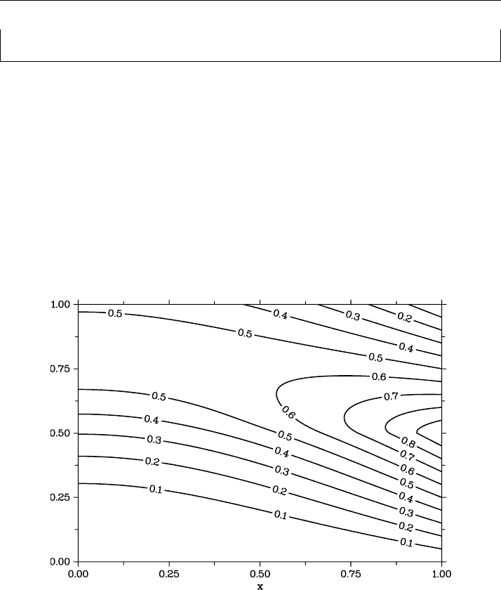
As the basic one, a uniform grid with h = 0.01 and τ = 0.01 for the problem with

l = 1 and T = 1 was used. In the realization of the quasi-real experiment for the direct

problem, the boundary condition at the right end point was set as follows:

ψ(t) =



2t/T , 0 < t < T/2,

2(T − t)/T, T/2 < t < T.

Figure 8.1 shows the contour lines for the direct-problem solution obtained with the

chosen boundary conditions.

Figure 8.1 Direct-problem solution

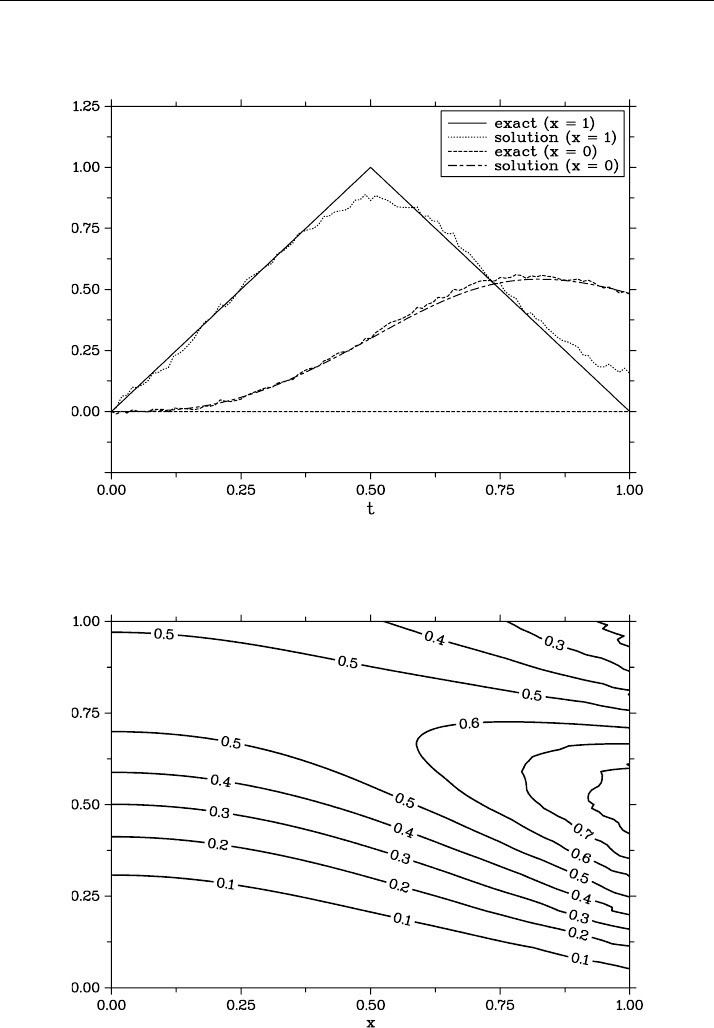
First of all, we would like to know how the inaccuracy in setting the boundary

conditions affects the solution accuracy in the inverse problem. Figure 8.2 shows the

solution of the inverse problem obtained with the inaccuracy level deﬁned by δ = 0.01.

Here, plotted are the exact and perturbed solutions at the left boundary (at x = 0),

serving the input data in solving the inverse problem. From these conditions, the

solution in the interval 0 < x ≤ l is to be reconstructed. Plotted in the ﬁgure are the

exact solution and the found solution at x = 1. The direct-problem solution at x = 1

for the found boundary condition is shown in Figure 8.3 (compare with Figure 8.1).

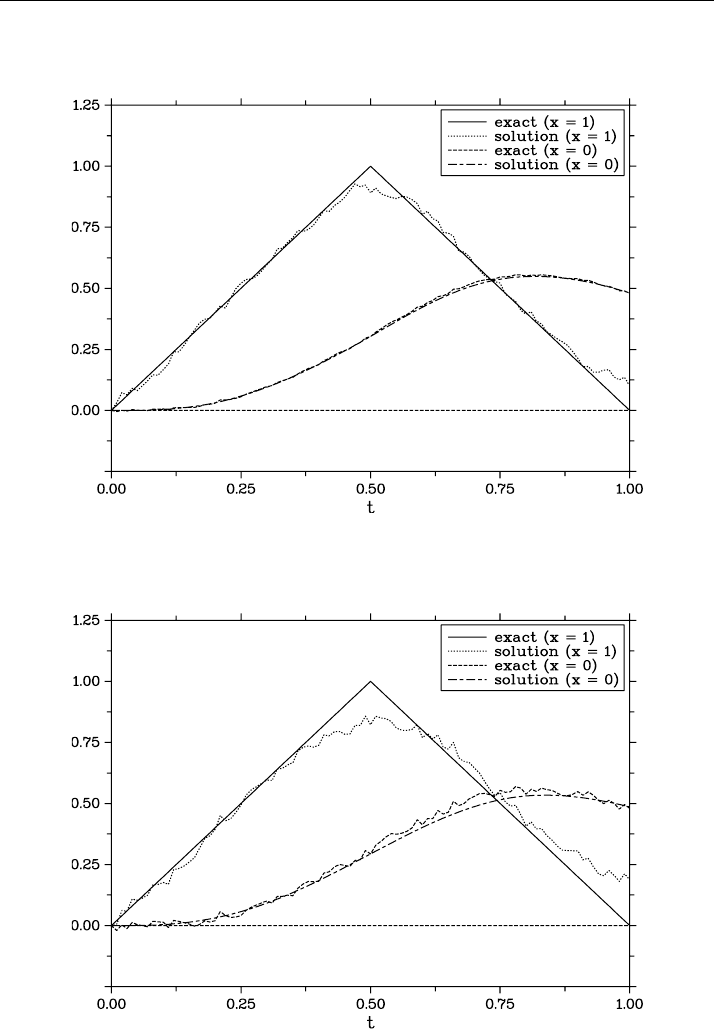
The effect due to the inaccuracy level is illustrated by Figures 8.4 and 8.5.

360 Chapter 8 Other problems

Figure 8.2 Inverse-problem solution obtained with δ = 0.01

Figure 8.3 Direct-problem solution obtained with the found boundary conditions

Section 8.1 Continuation over spatial variable in boundary value inverse problems 361

Figure 8.4 Inverse-problem solution obtained with δ = 0.005

Figure 8.5 Inverse-problem solution obtained with δ = 0.02

362 Chapter 8 Other problems

8.2 Non-local distribution of boundary conditions

For the approximate solution of the boundary value inverse problem for the one-

dimensional parabolic equation, a computational algorithm is often used based on

non-local perturbation of the boundary condition. This approach can be related to

the local Tikhonov regularization.

8.2.1 Model problem

We assume that the process of interest obeys the one-dimensional parabolic equation

of the second order. The related direct problem can be formulated as follows:

The solution u(x, t) is to be determined in the rectangle

=  × [0, T ],  ={x | 0 ≤ x ≤ l}, 0 ≤ t ≤ T.

The function u(x, t) satisﬁes the equation

∂u

∂t

∂

∂x



k(x)

∂u

∂x



, 0 < x < l, 0 < t ≤ T, (8.49)

with the usual constraints k(x) ≥ κ>0. The adopted boundary and initial conditions

are as follows:

k(x)

∂u

∂x

(0, t) = 0, 0 < t ≤ T, (8.50)

u(l, t) = ψ(t), 0 < t ≤ T, (8.51)

u(x, 0) = 0, 0 ≤ x ≤ l. (8.52)

We consider the boundary value inverse problem in which the boundary condition at

the right boundary is not given (the function ψ(t) in (8.51) is unknown). Instead, given

is the additional condition at the left boundary:

u(0, t) = ϕ(t), 0 < t ≤ T. (8.53)

Additionally, we assume that, as it is often the case in practice, the latter boundary

condition is given with some inaccuracy.

8.2.2 Non-local boundary value problem

Among the various possible approaches to the approximate solution of inverse prob-

lems for evolutionary equations, we choose to treat methods with perturbed initial

equation and methods with perturbed initial (boundary) conditions. The variant of the

generalized inverse method with the passage to a well-posed problem for a perturbed

equation was realized above by considering the spatial variable as the evolutionary

variable. It is of interest here to use the variant of this method with perturbed boundary

(initial, with the interpretation of the variable x as the evolutionary variable) condition.

Section 8.2 Non-local distribution of boundary conditions 363

We denote the approximate solution of the boundary value inverse problem (8.49),

(8.50), (8.52), (8.53) as u

(x, t) and determine it from the equation

∂u

∂t

∂

∂x



k(x)

∂u

∂x



, 0 < x < l, 0 < t ≤ T. (8.54)

We leave the boundary condition (8.50) and the initial condition (8.52) unchanged:

k(x)

∂u

∂x

(0, t) = 0, 0 < t ≤ T, (8.55)

(x, 0) = 0, 0 ≤ x ≤ l. (8.56)

We replace the boundary condition (8.53), which makes the inverse problem (8.49),

(8.50), (8.52), (8.53) an ill-posed problem, with the following non-local condition:

(0, t) + αu

(l, t) = ϕ(t), 0 < t ≤ T. (8.57)

In (8.54)–(8.57), the passage to a non-local boundary value problem can be made

immediately. A second possibility in formulating such a non-classical problem is

based on the consideration of the Tikhonov regularization method for problem (8.54)–

(8.57) interpreted as a boundary control problem (the boundary condition at the right

end point is (8.51)) with boundary observation (at the left end point, the condition

(8.53) is adopted). Next, we can try to formulate a related Euler equation, which, as

we saw, leads to non-classical boundary value problems. What is necessary is to only

take the fact into account that in the case of interest both for the ground and conjugate

states we have evolutionary problems with non-selfadjoint operators.

8.2.3 Local regularization

As it was repeated over and over again, in the application of regularization methods to

evolutionary problems we have two possibilities. In global regularization methods the

solution is to be determined at all times simultaneously, whereas in local regularization

methods the solution depends only on the pre-history, and can be determined sequen-

tially at separate times. Local regularization methods take into account the speciﬁc

feature of inverse problems for evolutionary problems in maximal possible measure.

Over time, we introduce the uniform grid

¯ω

={t

= nτ, n = 0, 1,...,N

,τN

= T },

and let u

(x) = u(x, t

). In the approximate solution of the inverse problem (8.54)–

(8.57), we perform the transition to the next time layer using the purely implicit scheme

364 Chapter 8 Other problems

for the direct problem:

n+1

− u

−

∂

∂x



k(x)

∂u

n+1

∂x



= 0, 0 < x < l, n = 0, 1,...,N

− 1, (8.58)

k(x)

∂u

n+1

∂x

(0) = 0, n = 0, 1,...,N

− 1, (8.59)

n+1

(l) = v

n+1

, n = 0, 1,...,N

− 1, (8.60)

(x) = 0, 0 ≤ x ≤ l. (8.61)

Using, on each time layer, the Tikhonov regularization for determining the boundary

condition at the right boundary (see (8.60)) implies minimization of the smoothing

functional

n+1

) = (u

n+1

(0) − ϕ

n+1

)

+ α(v

n+1

)

. (8.62)

Let us show that the minimization problem for the functional (8.62) under constraints

(8.58)–(8.61) is in fact equivalent to solving the difference problem with non-local

boundary conditions of type (8.57) on each time layer.

We represent the solution of problem (8.58)–(8.60) in the form

n+1

(x) = z

n+1

(x) + w

n+1

(x). (8.63)

In the latter representation, z

n+1

(x) is the solution of the difference problem

n+1

− u

−

∂

∂x



k(x)

∂z

n+1

∂x



= 0, 0 < x < l, n = 0, 1,...,N

− 1, (8.64)

k(x)

∂z

n+1

∂x

(0) = 0, n = 0, 1,...,N

− 1, (8.65)

n+1

(l) = 0, n = 0, 1,...,N

− 1, (8.66)

(x) = 0, 0 ≤ x ≤ l. (8.67)

Thereby, z

n+1

(x) is the solution of the direct problem with homogeneous condition of

the ﬁrst kind at the right boundary.

From (8.63) and (8.64)–(8.67), for w

n+1

(x) we obtain:

n+1

−

∂

∂x



k(x)

∂w

n+1

∂x



= 0, 0 < x < l, n = 0, 1,...,N

− 1, (8.68)

k(x)

∂w

n+1

∂x

(0, t) = 0, n = 0, 1,...,N

− 1, (8.69)

n+1

(l) = v

n+1

, n = 0, 1,...,N

− 1, (8.70)

(x) = 0, 0 ≤ x ≤ l. (8.71)

Taking into account the linearity of the coefﬁcient k(x) and its independence of time,

for the solution of the difference problem (8.68)–(8.71) we obtain the representation

n+1

(x) = q(x)v

n+1

, (8.72)

Section 8.2 Non-local distribution of boundary conditions 365

in which q(x) is the solution of the difference problem

−



k(x)



= 0, 0 < x < l, (8.73)

k(x)

(0) = 0, q(l) = 1. (8.74)

Substitution of (8.63) and (8.72) into (8.62) yields:

n+1

) = (z

n+1

(0) + q(0)v

n+1

− ϕ

n+1

)

+ α(v

n+1

)

. (8.75)

The minimum of (8.75) is attained at

n+1

(0) + q(0)v

n+1

− ϕ

n+1

))q(0) + αv

n+1

= 0. (8.76)

Thereby, for the boundary condition at the right boundary we have:

n+1

= q(0)

n+1

− z

n+1

(0)

α + q

(0)

. (8.77)

In the local regularization algorithm as applied to the solution of the inverse prob-

lem (8.54)–(8.57), the transition to the next time layer implies the solution of the direct

problems (8.64)–(8.67) and (8.73), (8.74), the calculation of the constant v

n+1

by for-

mula (8.76), and the use of representation (8.63), (8.72) for the solution of the inverse

problem.

Using the maximum principle for problem (8.64)–(8.67), we have q(0)>0; hence,

the condition (8.76) can be brought (see (8.70)) to the form

n+1

(0) +

q(0)

n+1

(l) = ϕ

n+1

. (8.78)

Thus, the minimization problem for the functional (8.62) under constraints (8.58)–

(8.61) is equivalent to the solution of the problem with the non-local boundary con-

ditions (8.58), (8.59), (8.61), and (8.77). With all these taken into account, we can

say that the local regularization algorithm is a discrete variant of the method with non-

locally perturbed boundary conditions (8.54)–(8.57) for the approximate solution of

the boundary value inverse problem (8.49), (8.50), (8.52), (8.53).

8.2.4 Difference non-local problem

To the differential problem with the non-local boundary condition (8.54)–(8.57), we

put in correspondence a difference problem. Along the spatial variable, we introduce

a uniform grid ¯ω with a grid size h over the interval

 = [0, l]:

¯ω ={x | x = x

= ih, i = 0, 1,...,N, Nh = l}.

In this grid, ω is the set of internal nodes, and ∂ω is the set of boundary nodes.