Schlick T. Molecular Modeling and Simulation: An Interdisciplinary Guide

Подождите немного. Документ загружается.

420 12. Monte Carlo Techniques

can be developed, as in the “end-transfer CB-MC” for chromatin, where one end

of the polymer is grown at the other end. Dramatic efﬁciency can be achieved –

quadratic vs. exponential scaling – in such applications [63].

A comparison of several biased MC schemes for small molecule design [224]

demonstrated the excellent performance of such methods compared to genetic

algorithms.

12.6.3 Hybrid MC

Exploiting Strengths of MC and MD

To enhance the efﬁciency of MC simulations, a simple idea emerged that attempts

to combine the favorable properties of molecular dynamics (MD) simulations —

sampling phase space in a directed manner guided by the shape of the energy

gradient — with that of MC — sampling phase space more globally. Ideally,

following conformation space by MD would generate a correct Boltzmann dis-

tribution of states, but the relatively short simulation lengths that are possible (see

MD chapters) imply local rather than global sampling.

This MC/MD combination [344, 347, 688] — moving some particles by MC

rules and others by MD, for example by combining global updates in position

space via MD with reasonable acceptance criteria by MC — can be more effective

for solvated biomolecular systems than either MC or MD alone. Such hybrid MC

methods have been very effective for small systems [575].

Overall Idea

For example, the ﬁrst step of a hybrid MC method can use a molecular dynamics

framework to specify the system’s candidate move: X[iΔt] −→ X[(i +1)Δt]

where Δt is the timestep. The MD algorithm must be time reversible and vol-

ume preserving so as to ensure detailed balance. The commonly used symplectic

Verlet method satisﬁes this requirement (see Chapters 13 and 14). Since the re-

cursive MD recipe relies on the velocities in addition to positions, the required

velocity vectors V = M

−1

P (P here designates momentum, not to be con-

fused with the symbol used earlier for probability) are generated from a Gaussian

distribution so as to obtain the target kinetic energy at the temperature T as-

suming energy equipartition. That is, the velocity components are drawn from a

Gaussian distribution proportional to the Boltzmann factor applied to the kinetic

energy:

ρ(P ) ∝ exp [−βE

(P )] . (12.46)

Following this MD-guided step, the second step of the hybrid MC method

applies the standard Metropolis acceptance criterion where the energy in the

Boltzmann factor is the Hamiltonian (potential plus kinetic energy). Namely,

the Metropolis criterion is applied to accept the new candidate

i+1

with

probability

12.6. Monte Carlo Applications to Molecular Systems 421

acc, HMC,ρ

=min



1, exp



−β



i+1

) − H(X

)



=min



exp [−βE

(

i+1

)] exp [−βE

(

i+1

)]

exp [−βE

)] exp [−βE

)]



=min



NVT

(

i+1

)exp[−βE

(

i+1

)]

NVT

)exp[−βE

)]



. (12.47)

Note that generalized ensembles can be emulated by HMC methods by ap-

plying weighting factors to the Metropolis-generated conﬁgurations. That is,

to sample from a general ensemble with μ(x) rather than ρ(x), we adjust the

acceptance criteria of eq. (12.47)tobe:

acc, HMC,μ

=min



μ(

i+1

)exp[−βE

(

i+1

)]

μ(X

)exp[−βE

)]



. (12.48)

The weighting must be accomplished to maintain detailed balance.

HMC methods have been quite successful for biomolecular sampling, and

many extensions to general ensembles and hybrid methods have been described.

See [15], for example, for a comparison of several HMC methods with various de-

tailed balance conditions, and [596] for a shadow HMC method which improves

sampling while adding modest computational cost.

12.6.4 Parallel Tempering and Other MC Variants

One idea that has gained popularity involves temperature jumps to accelerate

sampling. This idea of replica exchange is similar to simulated annealing but

here multiple simulations of non-interacting systems are involved [508, 1237].

Speciﬁcally, replicas (multiple copies) of the system that do not interact with one

another are simulated at different temperatures, and systems from different en-

sembles are periodically exchanged with a transition probability that maintains

each temperature’s equilibrium ensemble distribution:

acc, MC−PT

=min[1, exp ((β

− β

)(E

− E

)) ] (12.49)

where β

=1/(k

REM, however, requires many parallel processors and a careful protocol of

ensemble exchange and parameter selection to obtain rapid sampling and conver-

gence. These issues have been addressed mostly in the dynamics analog of REM

termed REMD. See a separate discussion of these issues in the MD chapters.

An energy-restricted multiple random walk MC protocol with similar advan-

tages to REM tempering in escaping from local barriers was introduced by Wang

& Landau [1328]. The method performs multiple random walks in energy space,

each to sample a different range of energy; the resulting information is combined

422 12. Monte Carlo Techniques

to produce canonical averages for calculating thermodynamic quantities at any

temperature. Both this method and REM perform similarly for protein conforma-

tional sampling and are faster by two orders of magnitude when compared to a

canonical MC simulation at a low temperature. However, the Wang/Landau MC

method was found to be easier to implement on single-processor systems, while

parallel tempering is advantageous for multi-processor machines [623].

Additional MC variants include Smart MC [1162], stochastic dynamics, um-

brella sampling, various methods that incorporate MC elements to enhance

barrier crossing events (e.g., the transition path sampling method of Chandler

and coworkers [147]), and potential-modiﬁcation approaches such as smoothing

and potential biasing techniques. See separate section for enhanced sampling and

recent reviews [1117,1117].

Given recent successes of MC methods for biomolecules [347,781,1457], some

advocate that recent improvements in MC methodology and increased computer

memory and speed lend support for the increased application of MC algorithms

for folding small biomolecules. Indeed, canonical, multi-canonical, biased MC

protocols that incorporate experimental information (e.g., knowledge-based di-

hedral angle distributions, and hybrids involving global optimization techniques

and MD) can signiﬁcantly enhance the sampling of low energy conﬁgurations and

reveal folding ensembles of small proteins.

General and ﬂexible MC modules have been built into standard programs like

CHARMM [575], with automatic optimization of step sizes and efﬁcient combi-

nations with minimization or MD modules. These optimized MC methods were

found to outperform standard Langevin dynamics simulations in reaching folded

states of small proteins.

In general, MC methods can become inefﬁcient for large systems but can

certainly be effective for coarse grained methods (e.g., chromatin folding [64,

1240]) and as vital components of other methods (e.g., transition path sampling

[147]). With increased usage and interest in coarse-grained models for larger

biomolecular complexes, further development of MC methods, including the

various extensions and hybrids described above, is warranted for biomolecular

applications as a whole.

There has been continued discussion on the relative merits of MC and MD for

biomolecules (e.g., [247, 619]). The limits of MD for simulating slow molecu-

lar events are clearly recognized, as is the high computational cost, though only

MD can ultimately yield detailed dynamic information such as folding pathways

and rates of conformational changes. Today, many enhanced sampling tools are

available (discussed separately). Thus, a practitioner is well-advised to use a com-

bination of MC, MD, local and global minimization algorithms, and enhanced

sampling approaches as appropriate, for the problems at hand.

12.6. Monte Carlo Applications to Molecular Systems 423

Molecular Dynamics: Basics

Chapter 13 Notation

YMBOL DEFINITION

Matrices

M mass matrix

pressure tensor (stress)

Vectors

g(X) constrained dynamics vector, components g

= r

− r

position vector for atom i

velocity vector component corresponding to atom i

force



acceleration (

X), or M

−1

F (X(t))

force on particle i due to all particles

V ,

velocity =

X (components {v

}), and its ﬁrst and second

time derivatives

initial velocity

position (components {x

}), and its ﬁrst and second

time derivatives

initial position

Lagrange multiplier vector for constrained dynamics

(components λ

)

∇E

energy gradient

Scalars & Functions

c speed of light

coordinate and velocity scaling parameters (for

constant pressure and temperature simulations)

Planck’s constant

particle mass

T. Schlick, Molecular Modeling and Simulation: An Interdisciplinary Guide, 425

Interdisciplinary Applied Mathematics 21, DOI 10.1007/978-1-4419-6351-2

13,

 Springer Science+Business Media, LLC 2010

426 13. Molecular Dynamics: Basics

Chapter 13 Notation Table (continued)

YMBOL DEFINITION

masses for ﬁctitious thermostat and barostat dynamic

variables

, r

interatomic distance and associated equilibrium value

velocity of the center of mass

dynamic variables for ﬁctitious thermostat and barostat

kinetic energy

potential energy



Hamiltonian and nearby Hamiltonian

number of atoms

number of degrees of freedom

P, P

pressure, target pressure

harmonic bond stretching constant

T, T

temperature, target temperature

isothermal compressibility

thermostat coupling parameter

δ(t)

Lyapunov exponent



trajectory perturbation

,ζ

thermodynamic coefﬁcients for constant pressure and

temperature simulations

wavelength (1/λ is wave number)

ν, ω

characteristic frequencies

volume variable

thermostat coupling parameter

Δt, Δt

, Δτ timesteps

Time is deﬁned so that motion looks simple.

John Archibald Wheeler, American theoretical physicist (1911–2008).

Molecular dynamics is clearly on the way to being a universal tool,

as if it were the differential calculus.

Sir John Royden Maddox [811], British science writer and Nature editor

(1925–2009).

13.1 Introduction: Statistical Mechanics by Numbers

13.1.1 Why Molecular Dynamics?

Molecular dynamics (MD) simulations represent the computer approach to sta-

tistical mechanics. As a counterpart to experiment, MD simulations are used to

estimate equilibrium and dynamic properties of complex systems that cannot be

calculated analytically. Representing the exciting interface between theory and

experiment, MD simulations occupy a venerable position at the crossroads of

mathematics, biology, chemistry, physics, and computer science.

13.1. Introduction: Statistical Mechanics by Numbers 427

The static view of a biomolecule, as obtained from X-ray crystallography for

example — while extremely valuable — is still insufﬁcient for understanding

a wide range of biological activity. It only provides an average, frozen view

of a complex system. Certainly, molecules are live entities, with their constituent

atoms continuously interacting among themselves and with their environment.

Their dynamic motions can explain the wide range of thermally-accessible states

of a system and thereby connect sequence to structure and function. Thus,

by following the dynamics of a molecular system in space and time, we can

obtain a rich amount of information concerning structural and dynamic proper-

ties. Though considered obvious today, relating motion to function of proteins

through sampling rugged energy landscapes was innovative when ﬁrst described

by Frauenfelder and Wolynes [422,1386].

Indeed, following the dynamics of molecular systems can provide valu-

able information concerning molecular geometries and energies; mean atomic

ﬂuctuations; local ﬂuctuations (like formation/breakage of hydrogen bonds,

water/solute/ion interaction patterns, or nucleic-acid backbone torsion motions);

rates of conﬁgurational changes (ring ﬂips, nucleic-acid sugar repuckering, diffu-

sion), enzyme/substrate binding; free energies; and the nature of various types

of concerted motions. Ultimately perhaps, large-scale deformations of macro-

molecules such as protein folding might be simulated, as discussed in the ﬁrst

chapter. This formidable aspect, however, is more likely to be an outgrowth of

hand-in-hand advances in both experiment and theory, not to speak of high-end

computing.

Though the MD approach remains popular because of its essential simplic-

ity and physical appeal (see below), it complements many other computational

tools for exploring molecular structures and properties, such as Monte Carlo sim-

ulations, Poisson-Boltzmann analyses, and energy minimization, as discussed in

preceding chapters, and Brownian dynamics and enhanced sampling methods, as

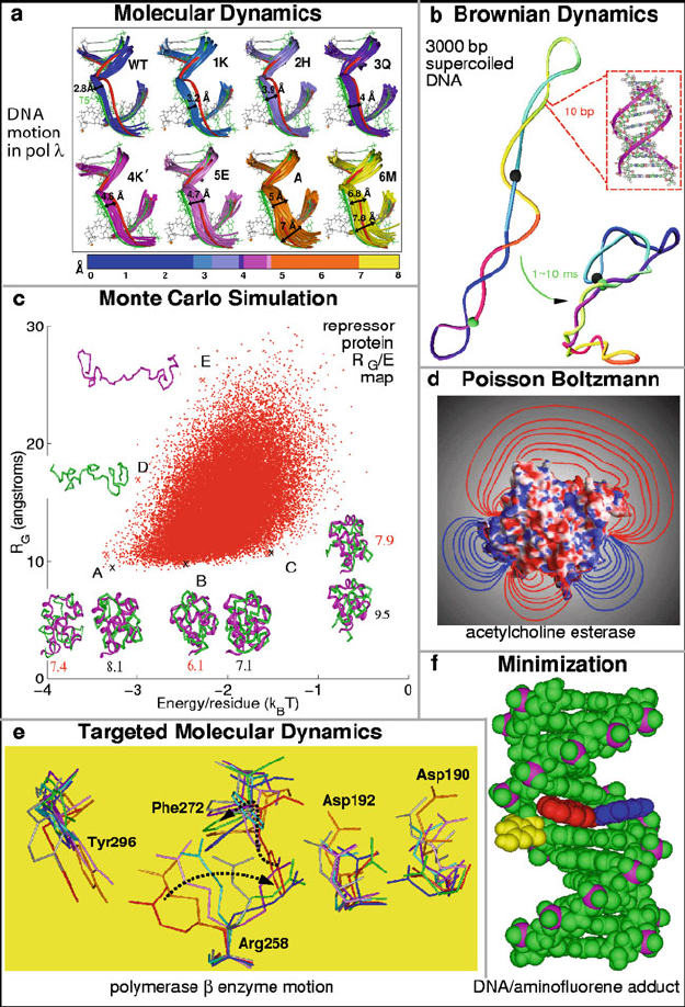
described in the next chapter. See examples in Table 13.1 and Figure 13.1. Each

technique is appropriate for a different class of problems.

13.1.2 Background

A solid grounding in classical statistical mechanics, thermodynamic ensembles,

time-correlation functions, and basic simulation protocols is essential for MD

practitioners. Such a background can be found, for example, in the books by

McQuarrie [853], Allen and Tildesley [22], and Frenkel and Smit [428]. Basic ele-

ments of simulation can be learned from the book of Ross [1067] and Bratley, Fox

and Schrage [165]. MD fundamentals, as well as advanced topics, are also avail-

able in texts by Allen and Tildesley [22], Frenkel and Smit [428] and Berenedsen

[122]. Basic introductions and useful examples in Gould and Tobochnik [474],

Rapaport [1038], Haile [494], and Field [398]. Some of these texts also describe

analysis tools for MD trajectories, a topic not considered here.

Good advanced texts for Hamiltonian dynamics and integration schemes are

those by Leimkuhler and Reich [731] and by Sanz-Serna and Calvo [1090]. Two

428 13. Molecular Dynamics: Basics

Table 13.1. Selected biomolecular sampling methods. Continuum solvation includes em-

pirical constructs, generalized Born models, stochastic dynamics, or Poisson Boltzmann

solutions, as discussed in Chapter 10. Targeted MD involves generating hypothetical paths

between two conformational endpoints [389]. See Figure 13.1 for illustrations.

Method Pros Cons CPU

• Molecular

Dynamics

(MD)

continuous motion, experimental bridge

between structures and macroscopic ki-

netic data

expensive; short

timespan

high

• Targeted

MD (TMD)

connection between two states; useful for

ruling out steric clashes and suggesting

high barriers

not necessarily physi-

cal

moderate

• Continuum

Solvation

mean-force potential approximates envi-

ronment and reduces model’s cost; useful

information on ionic atmosphere and

intermolecular associations

approximate moderate

• Brownian

Dynamics

(BD)

large-scale and long-time motion approximate hydrody-

namics; limited to sys-

tems with small inertia

moderate

• Monte Carlo

(MC)

large-scale sampling; useful statistics move deﬁnitions are

difﬁcult; unphysical

paths

low

•

Minimization

valuable equilibria information; experi-

mental constraints can be incorporated

no dynamic informa-

tion

low

books written in the early days of biomolecular simulations are by McCammon

and Harvey [846] and by Brooks, Pettitt and Karplus [178]. And there are always

good reviews of MD from time to time (e.g., [4,636,658]).

Given these many sources for the theory and application of MD simulations,

the focus in this chapter and the next is on providing a broad introduction

into the computational difﬁculties of biomolecular MD simulations and some

long-time integration approaches to these important problems. The reader is

advised to complement these aspects with the more standard topics available

elsewhere.

13.1.3 Outline of MD Chapters

We begin by describing in Section 13.2 the roots of molecular dynamics in

Laplace’s 19th-century vision. We then describe two basic limitations of Newto-

nian (classical) mechanics: determinism, and failure to capture quantum effects

(or electronic motion). We elaborate on the latter by noting that the classical

physics approximation is especially poor at lower temperatures and/or higher fre-

quencies. Section 13.3 discusses general issues in molecular and biomolecular

dynamics simulations, such as setting up the system (initial conditions, solvent

and ions, equilibration), estimating temperature, and other simple aspects of

the simulation protocol (equilibration, nonbonded interaction handling). We also

13.2. Laplace’s Vision of Newtonian Mechanics 429

elaborate upon the inherent chaotic (but bounded) behavior of biomolecules ﬁrst

mentioned in Section 13.2 by demonstrating sensitivity to initial conditions. We

motivate various methods for reducing the computational time of dynamic simu-

lations by emphasizing the large computational times required for biomolecules,

as well as extensive data-analysis and graphical requirements associated with the

voluminous data that are generated.

Given the large computational requirements, we introducein the same overview

section the concepts of accuracy, stability, symplecticness, and multiple-timesteps

(MTS) that are key to developing numerical integration techniques for biomolec-

ular dynamics simulations. In this context, we also mention constrained dynamics

and rigid-body approximations.

Though we refer to several of the methods in this introductory section (Section

13.3) that we only deﬁne later, a detailed understandingis not needed for grasping

the essentials that are communicated here. I recommend that students re-read

Section 13.3 after completing the two MD chapters.

Section 13.4 describes the symplectic Verlet/St¨ormer method and develops

its variants known as leapfrog, velocity Verlet, and position Verlet. This ma-

terial is followed by extension of Verlet to constrained dynamics formulations

(Section 13.5) and a reference to various MD ensembles (Section 13.6).

The next chapter introduces more advanced topics on various integration ap-

proaches for biomolecular dynamics; the material is suitable for students with

a good mathematical background. Speciﬁcally, we discuss symplectic integra-

tion methods, MTS (or force splitting) methods — via extrapolation and impulse

splitting techniques — and introduce the notion of resonance artifacts. Enhanc-

ing our understanding of resonance artifacts in recent years has been important

for developing large-timestep methods for MD. We continue to describe methods

for Langevin dynamics, Brownian dynamics, implicit integration, and enhanced

sampling.

13.2 Laplace’s Vision of Newtonian Mechanics

13.2.1 The Dream Becomes Reality

Besides “statistical mechanics by numbers”, I like to term MD as “Laplace’s

vision of Newtonian mechanics on supercomputers”.

Sir Isaac Newton (1642–1727) described in 1687 in his Principia masterpiece

(PhilosophiaeNaturalis Principia Mathematica) the grand synthesis of basic con-

cepts involving force and motion. This achievement was made possible by the

large pillars of empirical data laid earlier by scientists who studied the motion

of celestial and earthly bodies: Galileo Galilei (1564–1642), Nicolas Copernicus

(1473–1543), Tycho Brahe (1546–1601), and Johannes Kepler (1571–1630).

Newton’s second law of motion — that a body’s acceleration equals the net force

divided by its mass — is the foundation for molecular dynamics.

430 13. Molecular Dynamics: Basics

Figure 13.1. Illustrative images for selected biomolecular sampling methods. See caption

on the following page.