Schulz M. Control Theory in Physics and Other Fields of Science: Concepts, Tools, and Applications
Подождите немного. Документ загружается.

References 277
12. A. Bloch: Murphy’s Law and Other Reasons Why Things Go Wrong (PSS Adult,
1977) 268
13. H. Dawid, A. Mehlmann: Complexity 1, 51 (1996) 271
14. J.C. Harsanyi, R. Selten: A General Theory of Equilibrium Selection in Games
(MIT Press, Cambridge, 1988) 271
15. R. Isaacs: Differential Games (Wiley, New York, 1965) 271
16. D.M. Kreps: Game Theory and Economic Modelling (Oxford University Press,
New York, 1990) 271
17. J.V. Neumann: Mathematische Annalen, 100 295 (1928) 274
18. J.V. Neumann, O. Morgenstern: Theory of Games and Economic Behavior
(Princeton University Press, Princeton, NJ, 1944) 274
19. A. Mehlmann: Wer gewinnt das Spiel? (Vieweg, Braunschweig, 1997) 276

10
Optimization Problems
10.1 Notations of Optimization Theory
10.1.1 Introduction
Several problems, for example Pontryagin’s maximum principle or the min-
imax problems of game theoretical approaches, require the determination of
an extremum of a given function. These are typical optimization problems.
Most of the instructive problems which have been presented in the previous
chapters were relatively simple. Since only few degrees of freedom are con-
sidered, these problems were solvable by empirical concepts or by standard
analytical methods.
However, the treatment of sufficiently complex structures often requires
specific techniques. In this case it will be helpful to know some basic consid-
erations of modern optimization theory.
Optimization methods are not unknown in physics. A standard example
is free energy problems of thermodynamics. Here the equilibrium state of a
system coupled with a well-defined heat bath is obtainable by the minimiza-
tion of free energy. But also many other physical applications have turned out
to be in fact optimization problems, for example the determination of quan-
tum mechanical ground states using variational principles, the investigation
of systems in random environments, or the folding principles of proteins.
The main link between control theory and classical optimization theory is
due to Pontryagin’s maximum principle. Considering the state X and the ad-
joint variables, the generalized momenta P as free parameters, the maximum
principle requires the maximization of the Hamiltonian
H = H(X, P, u)=H(u) → max (10.1)
with respect to the n-component control u. The standard way of solving this
problem is a search for extremal solutions
∂H(u
∗
)
∂u
∗
= 0 (10.2)
M. Schulz: Control Theory in Physics and other Fields of Science
STMP 215, 279–293 (2006)
c
Springer-Verlag Berlin Heidelberg 2006
280 10 Optimization Problems
and, as a subsequent step, the decision if one of these solutions corresponds to
the global maximum or not. Unfortunately, this problem becomes much more
complicated if the control u should satisfy several constraints. For instance,
the control vector u can be restricted to a region G of the complete control
space U,oru has only discrete values.
10.1.2 Convex Objects
Convex Sets
The convexity of sets plays an important role in the optimization theory. In
the above introduced case we have to check if the region G forms a convex set.
The convexity is a very helpful property for many optimization problems. In
particular, the theory of optimization on convex sets is well established [1]. The
convexity of a region G requires that for each set of P points
u
(1)
,...,u
(P )
with u
(i)
∈ G (i =1,...,P), the linear form
v =
P
i=1
λ
i
u
(i)
(10.3)
with the real numbers λ
i
≥ 0and
P
i=1
λ
i
= 1 (10.4)
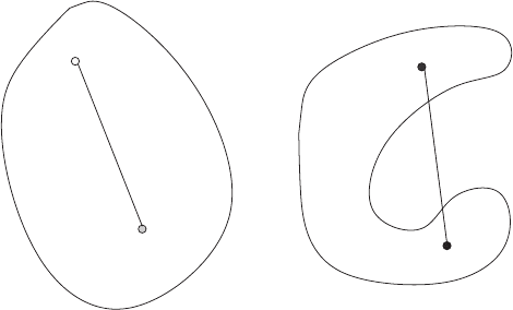
is also an element of G, i.e., v ∈ G, see Fig. 10.1. The verification of if a
region is convex or not is not trivial. A special situation occurs if the region
is described by a set of L linear inequalities of the type
(b)
(a)
Fig. 10.1. Convex (a) and nonconvex (b) sets. Each line between two points of a
convex set is also a subset of the convex set, while a line between two points of a
nonconvex set is not necessarily a subset of the nonconvex set

10.1 Notations of Optimization Theory 281
n
β=1
G
αβ
u
β
≤ g
α
with α =1,...,L (10.5)
or in a more compact form, by
Gu ≤ g (10.6)
with the L ×n matrix G and the L-component vector g. In this case, we may
replace u by a linear combination
u = λu
(1)
+(1− λ)u
(2)
with 0 ≤ λ ≤ 1 (10.7)
of two points u
(1)
and u
(2)
both satisfying (10.6). Thus, we obtain
Gu = G
λu
(1)
+(1− λ)u
(2)
= λGu
(1)
+(1− λ)Gu
(2)
≤ λg +(1− λ)g = g (10.8)
Regions which are defined by (10.6) are called convex polyhedrons.
Convex Functions
The decision if a local extremum u
∗
of a function H(u) is also a global min-
imum (or maximum) often needs special investigations. A helpful situation
occurs if the function is convex. A function H(u) over a region G is denoted
to be convex if for each pair
u
(1)
,u
(2)
of points with u
(i)
∈ G (i =1, 2) and
for each λ with 0 ≤ λ ≤ 1 the relation
H(λu
(1)
+(1− λ)u
(2)
) ≤ λH(u
(1)
)+(1− λ)H(u
(2)
) (10.9)
holds. Obviously, this definition requires that the convex function
1
must be
declared over a convex region. A sufficient condition that a function is convex
over a certain region G is that the Hesse matrix
H =
∂
2
H (u)
∂u
α
∂u
β
(10.10)
is positive definite for all points u ∈ G. Unfortunately, this condition requires
the computation of all eigenvalues or equivalently of all submatrices of H
and the subsequent proof that these quantities are positive. That is a very
expansive procedure, especially in the case of higher dimensional variables u.
An important property of convex function is the relation to its tangent planes.
It is simple to check by using (10.9) that
H(u) ≥ H(u
(0)
)+
∂H(u
(0)
)
∂u
(0)
(u − u
(0)
)foru, u
(0)
∈ G (10.11)
1
Convex functions correspond to a global minimum. In case we are interested in
a local maximum, we may consider concave functions or we can change the sign
of the function. The latter step implies an exchange of minimum and maximum
points.

282 10 Optimization Problems
i.e., a convex function always lies above its tangent planes. A local minimum
of a convex function H(u) over a convex region G is always the global min-
imum. This statement follows directly from (10.11) by identifying u
(0)
with
the position of the minimum. Thus we have ∂H(u
(0)
)/∂u
(0)
= 0 and therefore
H(u) ≥ H(u
(0)
) for all u ∈ G.
Linear functions H(u)=cu + d with the n-dimensional vector c and the
scalar d are always convex
2
. Quadratic functions
H(u)=
1
2
uCu + cu + d (10.12)
are convex if the symmetric matrix C of type n × n is positive definite. Al-
though these classes of functions seem to be very special, they play an impor-
tant role in control theoretical problems. Recall that the Hamiltonian of many
control problems is often a linear function of the control variable u, especially
if the performance does not depend on u. Furthermore, linear quadratic prob-
lems also lead to functions H(u) which are elements of this special set of
functions.
10.2 Optimization Methods
10.2.1 Extremal Solutions Without Constraints
The simplest case of an optimization problem occurs if the function H(u)is
a continuous function declared over a certain region G of the control space.
Then, either the possible candidates for the global minimum (maximum) are
the solutions of the extremal equation
∂H(u)
∂u
= 0 (10.13)
or the minimum (maximum) is located at the boundary ∂G of the region G.
The solution of the n usually nonlinear equations can be realized by analytic
methods only if the dimension of the problem, n, is very low or if the func-
tion H(u) is very simple. Especially the two classes of linear and quadratic
functions are of special interest. Since a linear function with the exception of
H(u) = const. has no extremal points, i.e., no solutions of (10.13), the opti-
mum is always located at the border of G. Here, we need the techniques of
linear optimization. The quadratic function (10.12) requires the solution of a
linear equation
Cu = −c (10.14)
This equation has for det C = 0 a unique solution, u
∗
= −C
−1
c.IfC is
positive definite and u
∗
∈ G, the optimization problem is solved.
2
And simultaneously also concave.

10.2 Optimization Methods 283
If the analytical solution of (10.13) fails, the application of numerical meth-
ods seems to be an alternative approach. Here, we distinguish between deter-
ministic methods and random techniques. An example for a deterministic
technique is Newton’s procedure. Here, we assume that u
(k)
is an approxima-
tion of the wanted extremum. Then, the expansion around this point up to
the second-order gives
H(u)≈H(u
(k)
)+
∂H(u
(k)
)
∂u
(k)
(u−u
(k)
)+
1
2
(u−u
(k)
)
∂
2
H(u
(k)
)
∂u
(k)
∂u
(k)
(u−u
(k)
)(10.15)
This is a quadratic form from which we can calculate straightforwardly the
corresponding extremum "u
∗
. However, because the right-hand side is only an
approximation of the complete function H(u), the solution "u
∗
is also only an
approximation of the true extremal point. On the other hand, "u
∗
is usually a
better approximation of the extremal point as u
(k)
. Thus, we may identify the
solution "u
∗
with u
(k+1)
and start the iteration procedure again with the new
input u
(k+1)
. Repeated application of this procedure may lead to a continuous
approach of u
(k)
to the true extremum u
∗
for k →∞.
Other traditional deterministic methods (see also [46]) are steepest descent
algorithms, subgradient methods [5], the Fletcher–Reeves algorithm [6]and
the Polak–Ribiere algorithm [7], trust region methods [6], or the coordinate
method in Hooke and Jeves [8, 9, 46].
Stochastic optimization methods [45] work usually without derivatives.
The idea is very simple. First, we choose a point
u ∈ G and determine H =
H(
u). Then, the region G is embedded in a hypercube C ⊃ G of dimension n
and unit length l. A randomly chosen set of n real numbers ξ
i
∈ [0,l] (with
i =1,...,n) is used to determine a point u
of the hypercube. If u ∈ G
and H(u) <
H,wesetu = u
and H = H(u
); otherwise u and H remain
unchanged. Repeated application of this algorithm then leads to a successive
improvement of the estimation u
∗
= u and H(u
∗
)=H.
Such algorithms require a random generator which produces uniformly dis-
tributed random numbers. Unfortunately, computer-generated random num-
bers are not really stochastic, since computer programs are deterministic al-
gorithm. But, given an initial number (generally called the seed) a number
of mathematical operations can be performed on the seed so as to generate
apparently unrelated pseudorandom numbers. The output of random number
generators is usually tested with various statistical methods to ensure that the
generated number series are really random in relation to one another. There
is an important caveat: if we use a seed more than once, we will get identical
random numbers every time. However, several commercial programs pull the
seed from somewhere within the system, so the seed is unlikely to be the same
for two different simulation runs.
A given random number algorithm generates a series of random num-
bers {η
1
,η
2
,...,η
N
} with a certain probability distribution function. If we
know this distribution function p
rand
(η), we now have from the rank ordering

284 10 Optimization Problems
statistics [10, 11] that the likely rank of a random number η in a series of N
numbers is
n = NP
<
(η)=N
η
−∞
dz p
rand
(z) . (10.16)
In other words, if the random generator creates random series which are dis-
tributed with p
rand
(η), the corresponding series {P
<
(η
1
),P
<
(η
2
) ,...,P
<
(η
N
)}
is uniformly distributed over the interval [0, 1]. Unfortunately, this concept
exhibits a slow rate of convergence. An alternative way is the application of
quasirandom sequences instead pseudorandom numbers [12, 13, 14, 15, 16, 17,
18, 19, 20]. The quasirandom sequences, sometimes also called low-discrepancy
sequences, usually permit us to improve the performance of the random al-
gorithms, offering shorter computational times and higher accuracy.
We remark that the low-discrepancy sequences are deterministic series,
so the popular notation quasirandom can be misleading. The discrepancy
property is a measure of uniformity for the distribution of the points. Let us
assume that the quasirandom process has generated Q points distributed over
the whole hyperspace. Then, the discrepancy is defined by
D
Q
=sup
R∈C
n(R)
Q
−
v(R)
l
n
(10.17)
where R is a spherical region of the hypercube, v(R) is the volume of this
region and n(R) is the number of points in this region. Obviously, the
discrepancy vanishes for Q →∞in case the of a homogeneous distribu-
tion of points over the whole hypercube. Mainly for the multidimensional
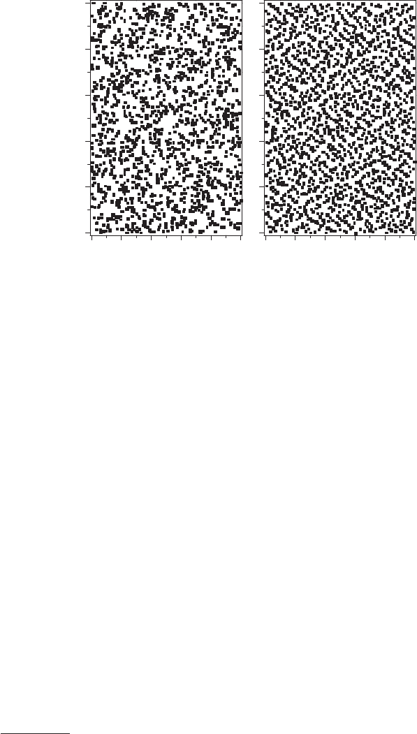
case, a low discrepancy corresponds to no large gaps and no clustering of
points in the hypercube (Fig. 10.2). Similar to a pseudorandom generator, a
quasirandom generator originates from the number theory. But in contrast to
the pseudorandom series, quasirandom sequences offer a pronounced deter-
ministic behavior. A quasirandom generator transforms an arbitrary positive
integer I into a quasirandom number ξ
I
via the following two steps. Firstly,
the integer I will be decomposed into the integer coefficients a
k
with respect
to the basis b
I =
∞
k=0
a
k
b
k
(10.18)
with 0 ≤ a
k
≤ b − 1. The coefficients form simply the representation of I
within the basis b. The second step is the computation of the quasirandom
number by the calculation of the sum
ξ
I
=
∞
k=0
a
k
b
−k−1
. (10.19)
10.2 Optimization Methods 285
0.0 0.2 0.4 0.6 0.8 1.0
0.0
0.2
0.4
0.6
0.8
1.0
y
0.0 0.2 0.4 0.6 0.8 1.0
xx
Fig. 10.2. Two-dimensional plot of pseudorandom number pairs (left)and
quasirandom number pairs (right). The quasirandom number series are created with
base 2 (x-axis) and with base 3 (y-axis)
For example, the first quasirandom numbers
3
corresponding to base 2 are 1/2,
1/4, 3/4, 1/8, 5/8,... while the sequence of base 3 starts with 1/3, 2/3, 1/9,
4/9, 7/9.
The merit of a quasirandom generator method is fast convergence. The
theoretical upper bound rate of convergence of the discrepancy is ln
n
Q/Q
where n is the dimension of the problem [21]. In contrast, the discrepancy of
a pseudo-random process converges as Q
−1/2
.
10.2.2 Extremal Solutions with Constraints
The standard version to determine the extremals of functions with µ con-
straints given by the equations
g
i
(u)=0 for i =1,...,µ (10.20)
is the Lagrange method. The Lagrange function
H
(u)=H(u)+
µ
i=1
λ
i
g
i
(u) (10.21)
can now be treated in the same way as the function H(u). The n extremal
equations together with the µ constraints form a system of usually nonlinear
equations for the µ Lagrange multipliers and the n components of u.Inprin-
ciple, the above discussed deterministic and stochastic numerical methods are
3
Corresponding to the integers I =1, 2, 3,....

286 10 Optimization Problems
also applicable for the determination of extremals under constraints. A special
feature is the penalty function method. Here, we construct a utility function
H(u, σ)=H(u)+σ g(u)
2
(10.22)
where g(u) is a suitable chosen norm with respect to the constraints. A
possible, but not necessary form is the Euclidian norm g
2
= g
2
1
+...+g
2
µ
.The
parameter σ is the penalty parameter, where σ>0 corresponds to a search
for a minimum while σ<0 is used for the determination of a maximum.
In principle, one can determine the minimum point of the function H(u, σ)
similar to the previous section. Let us assume that a minimum point was
found to be u
∗
(σ). It can be demonstrated [22]thatfor0<σ
1
<σ
2
the three
relations hold
H(u
∗
(σ
1
),σ
1
) ≤ H(u
∗
(σ
2
),σ
2
) (10.23)
g(u(σ
1
))
2
≥g(u(σ
2
))
2
(10.24)
and
H(u
∗
(σ
1
)) ≥ H(u
∗
(σ
2
)) (10.25)
Hence, it may be expected that for a series σ
i
→∞the value of u
∗
(σ
i
)
converges to the new minimum point considering the constraints.
10.2.3 Linear Programming
Linear programming deals with the optimization of linear problems. Such
problems are typical for the application of Pontryagin’s maximum principle to
physical systems controlled by external forces and a performance independent
of the control
4
. In fact, the equations of motion of such systems are given by
˙
X =
"
F (X, t)+u (10.26)
Thus, the Hamiltonian (2.94) reads
H (t, X, P, u)=P
"
F (X, t)+uP − φ(t, X) (10.27)
and the optimization problem involves the determination of the maximum of
H(u)=H
0
+ uP (10.28)
In this case the maximum is at the boundary ∂G of the admissible region G of
control states u. Furthermore, if this region is defined by a set of inequalities
G = {u ∈ U | Gu ≤ g and u ≥ 0}⊂U (10.29)
the global maximum is reached for one of the corners of the polyhedron de-
fined by (10.29). If the region is convex, the maximum can be found by the
4
This is typical for an optimal time problem or an endpoint performance (Meier
problem).
10.2 Optimization Methods 287
simplex algorithm [23, 24, 22, 25, 26]. In principle, this algorithm starts from
a randomly chosen corner u
(k)
with the initial label k = 0. Then, a second
corner u
is chosen, so that (i) u
is the topological neighbor of u
(k)
and (ii)
H(u
) >H(u
(k)
). If such a corner was found, we set u
(k+1)
= u
and repeat
the algorithm. If no further u
can be detected so that both conditions are
fulfilled, the currently reached corner corresponds to the global maximum so-
lution. If the set G is nonconvex, it may be possible to separate the region
to exhaustive and mutually exclusive convex subsets G
i
and solve the linear
programming problem for each G
i
separately. The global maximum is then
the maximum of all local maxima related to the subsets.
10.2.4 Combinatorial Optimization Problems
If the control state has only discrete values, we speak about a combinatorial
optimization problem. Such problems play an important role for several tech-
nological and physical applications. A standard example is the so-called Ising
model. Usually, the Ising model is described by a physical is described by a
physical Hamiltonian given by
H = H
0
(X)+
n
i,j=1
J
ij
(X)S
i
S
j
+
n
i=1
B
i
S
j
(10.30)
where S
i
are the discrete spin variables, and B
i
is denoted as the local field
and J
ij
as the coupling constants. The physical standard problem is the de-
termination of the ground state of H or alternatively, the thermodynamical
weight of a spin configuration {S
1
,...,S
i
,...}. This is of course a repeatedly
investigated problem in the context of spin glasses [27, 28, 29, 30, 31, 32],
protein folding [33, 34, 35], or phase transitions in spin systems [36, 37, 38]
and it is strongly connected with the concept of optimization. However, this
is no real control problem.
But a control problem occurs if we are interested in the inverse situation.
Usually, the physical degrees of freedom represented by the spin variables S
i
are coupled with another set of internal degrees of freedom X. These quanti-
ties are assumed to be passive for the above mentioned spin dynamics, i.e., X
determines the coupling constants J
ij
(X) and the spin-independent contribu-
tion H
0
(X), but for a given physical problem X is assumed to be fixed. But
we may also ask for the dynamics of X under a certain spin configuration.
Then, the Hamiltonian (10.30), leads to evolution equations of the form
˙
X = F
(0)
(X)+
n
i,j=1
F
(1)
ij
(X)S
i
S
j
(10.31)
where we may identify the discrete spin variables as components of the n-
component control u. From here, we obtain, for example via the deterministic
Hamiltonian (2.94) or the corresponding stochastic version (7.65) a classical
combinatorial optimization problem.