Stewart J. Calculus

Подождите немного. Документ загружается.

602

Perhaps the most important of all the applications of calculus is to differential equa-

tions. When physical scientists or social scientists use calculus, more often than not

it is to analyze a differential equation that has arisen in the process of modeling some

phenomenon that they are studying. Although it is often impossible to ﬁnd an explicit

formula for the solution of a differential equation, we will see that graphical and numer-

ical approaches provide the needed information.

Direction ﬁelds enable us

to sketch solutions of

differential equations with-

out an explicit formula.

DIFFERENTIAL

EQUATIONS

MODELING WITH DIFFERENTIAL EQUATIONS

In describing the process of modeling in Section 1.2, we talked about formulating a math-

ematical model of a real-world problem either through intuitive reasoning about the phe-

nomenon or from a physical law based on evidence from experiments. The mathematical

model often takes the form of a differential equation, that is, an equation that contains an

unknown function and some of its derivatives. This is not surprising because in a real-

world problem we often notice that changes occur and we want to predict future behavior

on the basis of how current values change. Let’s begin by examining several examples of

how differential equations arise when we model physical phenomena.

MODELS OF POPULATION GROWTH

One model for the growth of a population is based on the assumption that the population

grows at a rate proportional to the size of the population. That is a reasonable assumption

for a population of bacteria or animals under ideal conditions (unlimited environment, ade-

quate nutrition, absence of predators, immunity from disease).

Let’s identify and name the variables in this model:

The rate of growth of the population is the derivative . So our assumption that the

rate of growth of the population is proportional to the population size is written as the

equation

where is the proportionality constant. Equation 1 is our ﬁrst model for population

growth; it is a differential equation because it contains an unknown function P and its

derivative .

Having formulated a model, let’s look at its consequences. If we rule out a population

of 0, then for all t. So, if , then Equation 1 shows that for all t.

This means that the population is always increasing. In fact, as increases, Equation 1

shows that becomes larger. In other words, the growth rate increases as the popula-

tion increases.

Equation 1 asks us to ﬁnd a function whose derivative is a constant multiple of itself.

We know from Chapter 3 that exponential functions have that property. In fact, if we let

, then

Thus any exponential function of the form is a solution of Equation 1. In Sec-

tion 10.4 we will see that there is no other solution.

Allowing C to vary through all the real numbers, we get the family of solutions

whose graphs are shown in Figure 1. But populations have only positive

values and so we are interested only in the solutions with . And we are probably con-C ! 0

P!t" ! Ce

P"!t" ! C!ke

" ! k!Ce

" ! kP!t"

P!t" ! Ce

dP#dt

P!t"

P"!t" ! 0k ! 0P!t" ! 0

dP#dt

! kP

dP#dt

P ! the number of individuals in the population !the dependent variable"

t ! time !the independent variable"

10.1

603

N Now is a good time to read (or reread) the dis-

cussion of mathematical modeling on page 24.

F I G U R E 1

The family of solutions of dP/dt=kP

cerned only with values of t greater than the initial time . Figure 2 shows the physi-

cally meaningful solutions. Putting , we get , so the constant C

turns out to be the initial population, .

Equation 1 is appropriate for modeling population growth under ideal conditions, but

we have to recognize that a more realistic model must reﬂect the fact that a given environ-

ment has limited resources. Many populations start by increasing in an exponential man-

ner, but the population levels off when it approaches its carrying capacity K (or decreases

toward K if it ever exceeds K). For a model to take into account both trends, we make two

assumptions:

if P is small (Initially, the growth rate is proportional to P.)

if (P decreases if it ever exceeds K.)

A simple expression that incorporates both assumptions is given by the equation

Notice that if P is small compared with K, then is close to 0 and so . If

, then is negative and so .

Equation 2 is called the logistic differential equation and was proposed by the Dutch

mathematical biologist Pierre-François Verhulst in the 1840s as a model for world popula-

tion growth. We will develop techniques that enable us to ﬁnd explicit solutions of the

logistic equation in Section 10.4, but for now we can deduce qualitative characteristics of

the solutions directly from Equation 2. We ﬁrst observe that the constant functions

and are solutions because, in either case, one of the factors on the right

side of Equation 2 is zero. (This certainly makes physical sense: If the population is ever

either 0 or at the carrying capacity, it stays that way.) These two constant solutions are

called equilibrium solutions.

If the initial population lies between 0 and K, then the right side of Equation 2 is

positive, so and the population increases. But if the population exceeds the car-

rying capacity , then is negative, so and the population

decreases. Notice that, in either case, if the population approaches the carrying capacity

, then , which means the population levels off. So we expect that the

solutions of the logistic differential equation have graphs that look something like the ones

in Figure 3. Notice that the graphs move away from the equilibrium solution and

move toward the equilibrium solution .

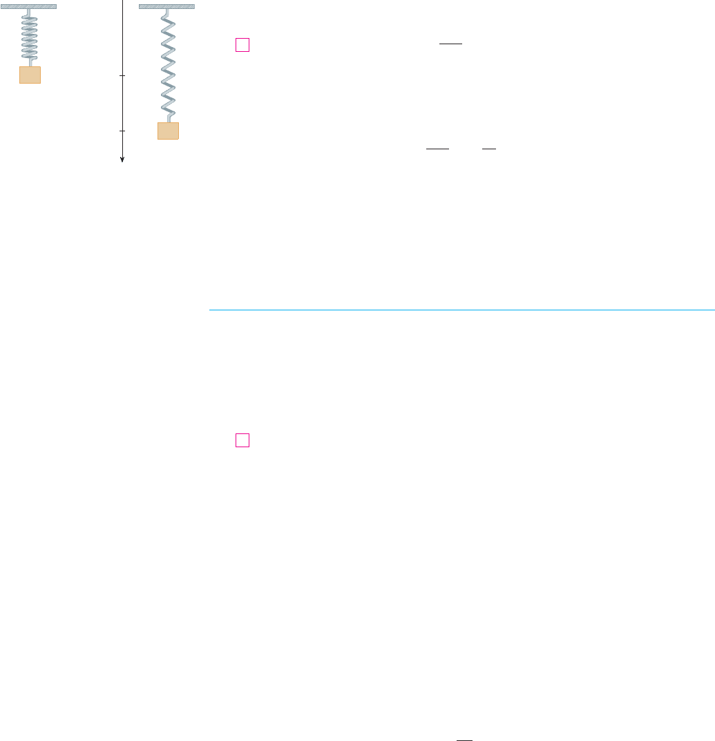
A MODEL FOR THE MOTION OF A SPRING

Let’s now look at an example of a model from the physical sciences. We consider the

motion of an object with mass m at the end of a vertical spring (as in Figure 4). In Sec-

tion 6.4 we discussed Hooke’s Law, which says that if the spring is stretched (or com-

pressed) x units from its natural length, then it exerts a force that is proportional to x:

where k is a positive constant (called the spring constant). If we ignore any external resist-

ing forces (due to air resistance or friction) then, by Newton’s Second Law (force equals

restoring force ! #kx

P ! K

P ! 0

dP#dt l 0!P l K"

dP#dt

01 # P#K!P ! K"

dP#dt ! 0

P!0"

P!t" ! KP!t" ! 0

dP#dt

01 # P#KP ! K

dP#dt $ kPP#K

! kP

1 #

P ! K

$ kP

P!0"

P!0" ! Ce

k!0"

! Ct ! 0

t ! 0

604

|| ||

CHAPTER 10 DIFFERENTIAL EQUATIONS

0 t

F I G U R E 2

The family of solutions P(t)=Ce

with C>0 and t˘0

F I G U R E 3

Solutions of the logistic equation

P=K

P =0

equilibrium

solutions

mass times acceleration), we have

This is an example of what is called a second-order differential equation because it

involves second derivatives. Let’s see what we can guess about the form of the solution

directly from the equation. We can rewrite Equation 3 in the form

which says that the second derivative of x is proportional to x but has the opposite sign. We

know two functions with this property, the sine and cosine functions. In fact, it turns

out that all solutions of Equation 3 can be written as combinations of certain sine

and cosine functions (see Exercise 4). This is not surprising; we expect the spring to oscil-

late about its equilibrium position and so it is natural to think that trigonometric functions

are involved.

GENERAL DIFFERENTIAL EQUATIONS

In general, a differential equation is an equation that contains an unknown function and

one or more of its derivatives. The order of a differential equation is the order of the high-

est derivative that occurs in the equation. Thus Equations 1 and 2 are ﬁrst-order equations

and Equation 3 is a second-order equation. In all three of those equations the independent

variable is called t and represents time, but in general the independent variable doesn’t

have to represent time. For example, when we consider the differential equation

it is understood that y is an unknown function of x.

A function is called a solution of a differential equation if the equation is satisﬁed

when and its derivatives are substituted into the equation. Thus is a solution of

Equation 4 if

for all values of x in some interval.

When we are asked to solve a differential equation we are expected to ﬁnd all possible

solutions of the equation. We have already solved some particularly simple differential

equations, namely, those of the form

For instance, we know that the general solution of the differential equation

is given by

where C is an arbitrary constant.

But, in general, solving a differential equation is not an easy matter. There is no sys-

tematic technique that enables us to solve all differential equations. In Section 10.2, how-

ever, we will see how to draw rough graphs of solutions even when we have no explicit

formula. We will also learn how to ﬁnd numerical approximations to solutions.

y !

% C

y" ! x

y" ! f !x"

f "!x" ! x f !x"

fy ! f !x"

y" ! xy

! #

! #kx

SECTION 10.1 MODELING WITH DIFFERENTIAL EQUATIONS

|| ||

605

F I G U R E 4

equilibrium

position

EXAMPLE 1 Show that every member of the family of functions

is a solution of the differential equation .

SOLUTION We use the Quotient Rule to differentiate the expression for y:

The right side of the differential equation becomes

Therefore, for every value of c, the given function is a solution of the differential

equation.

When applying differential equations, we are usually not as interested in ﬁnding a fam-

ily of solutions (the general solution) as we are in ﬁnding a solution that satisﬁes some

additional requirement. In many physical problems we need to ﬁnd the particular solution

that satisﬁes a condition of the form . This is called an initial condition, and the

problem of ﬁnding a solution of the differential equation that satisﬁes the initial condition

is called an initial-value problem.

Geometrically, when we impose an initial condition, we look at the family of solution

curves and pick the one that passes through the point . Physically, this corresponds

to measuring the state of a system at time and using the solution of the initial-value prob-

lem to predict the future behavior of the system.

EXAMPLE 2 Find a solution of the differential equation that satisﬁes

the initial condition .

SOLUTION Substituting the values and into the formula

from Example 1, we get

Solving this equation for c, we get , which gives . So the solution

of the initial-value problem is

y !

1 %

1 #

3 % e

3 # e

c !

2 # 2c ! 1 % c

2 !

1 % ce

1 # ce

1 % c

1 # c

y !

1 % ce

1 # ce

y ! 2t ! 0

y!0" ! 2

y" !

# 1"

, y

y!t

" ! y

4ce

!1 # ce

2ce

!1 # ce

# 1" !

1 % ce

1 # ce

# 1

(

!1 % ce

# !1 # ce

!1 # ce

(

# c

% ce

% c

!1 # ce

2ce

!1 # ce

y" !

!1 # ce

"!ce

" # !1 % ce

"!#ce

!1 # ce

y" !

# 1"

y !

1 % ce

1 # ce

606

|| ||

CHAPTER 10 DIFFERENTIAL EQUATIONS

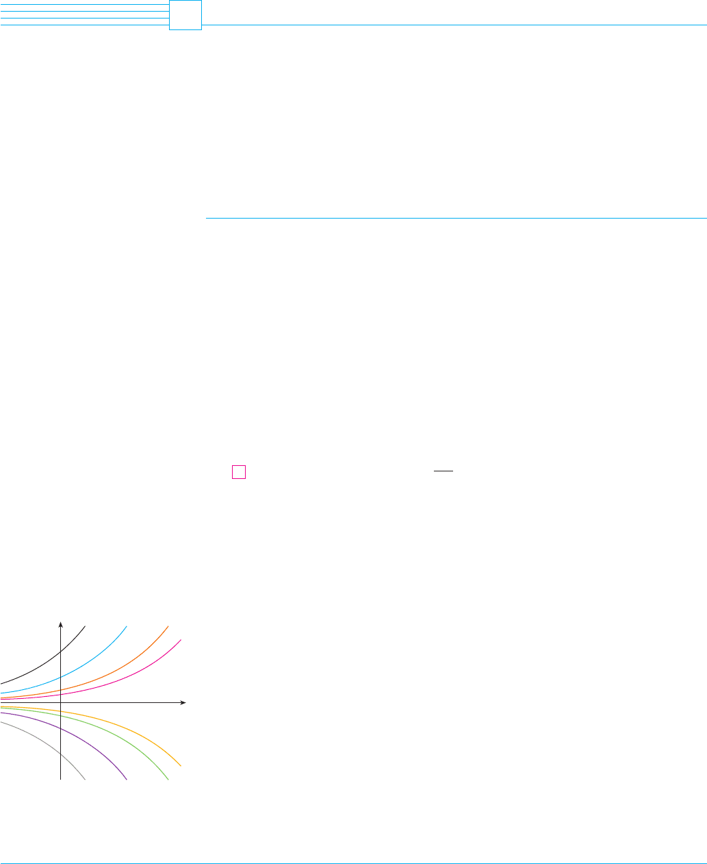
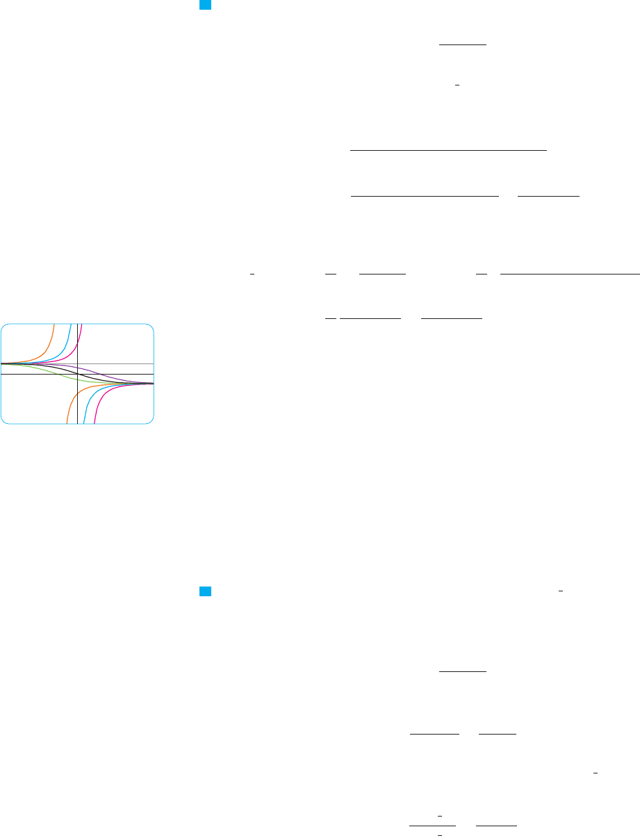
N Figure 5 shows graphs of seven members of

the family in Example 1. The differential equation

shows that if , then . That is

borne out by the ﬂatness of the graphs near

and .y ! #1y ! 1

y" $ 0y $ &1

_5 5

F I G U R E 5

SECTION 10.1 MODELING WITH DIFFERENTIAL EQUATIONS

|| ||

607

A population is modeled by the differential equation

(a) For what values of is the population increasing?

(b) For what values of is the population decreasing?

10. A function satisﬁes the differential equation

(a) What are the constant solutions of the equation?

(b) For what values of is increasing?

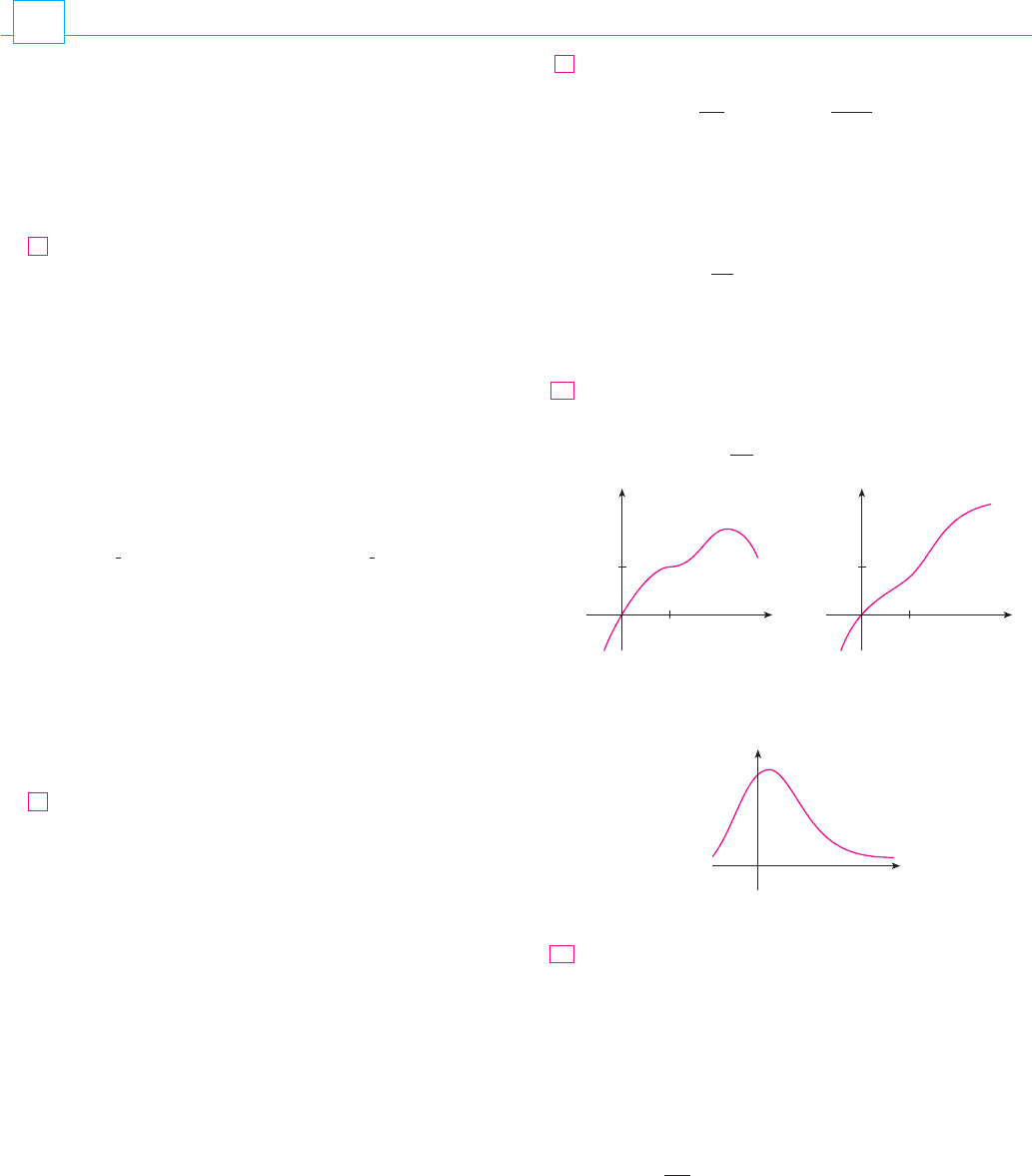
Explain why the functions with the given graphs can’t be

solutions of the differential equation

12. The function with the given graph is a solution of one of the

following differential equations. Decide which is the correct

equation and justify your answer.

A. B. C.

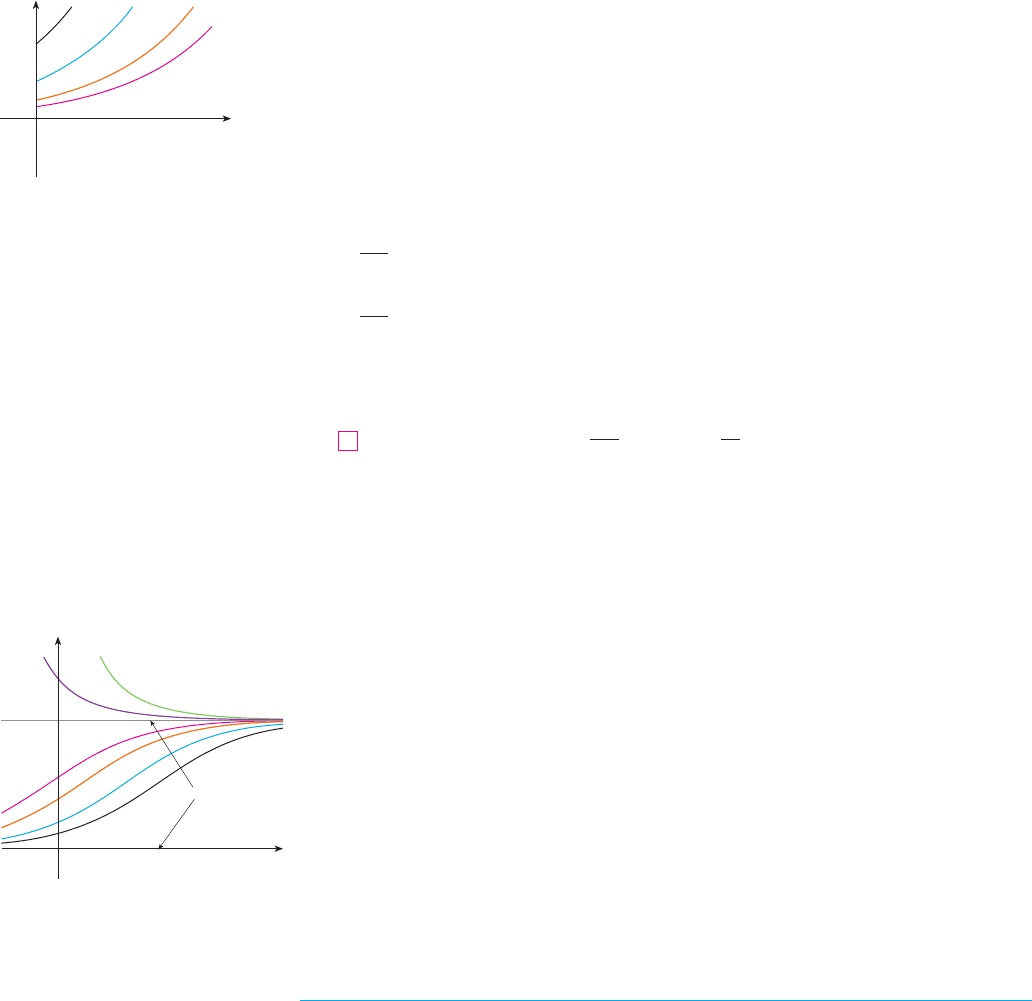
Psychologists interested in learning theory study learning

curves. A learning curve is the graph of a function , the

performance of someone learning a skill as a function of the

training time . The derivative represents the rate at

which performance improves.

(a) When do you think increases most rapidly? What hap-

pens to as increases? Explain.

(b) If is the maximum level of performance of which the

learner is capable, explain why the differential equation

is a reasonable model for learning.

k a positive constant

! k!M # P"

tdP#dt

dP#dtt

P!t"

13.

y" ! 1 # 2xyy" ! #2xyy" ! 1 % xy

0 x

(a) (b)

! e

!y # 1"

11.

! y

# 6y

% 5y

y!t"

! 1.2P

1 #

4200

1. Show that is a solution of the differential equa-

tion .

2. Verify that is a solution of the

initial-value problem

on the interval .

(a) For what values of does the function satisfy the

differential equation ?

(b) If and are the values of that you found in part (a),

show that every member of the family of functions

is also a solution.

4. (a) For what values of does the function satisfy

the differential equation ?

(b) For those values of , verify that every member of the

family of functions is also a

solution.

5. Which of the following functions are solutions of the differ-

ential equation ?

(a) (b)

6. (a) Show that every member of the family of functions

is a solution of the differential equation

;

(b) Illustrate part (a) by graphing several members of the

family of solutions on a common screen.

the initial condition .

(d) Find a solution of the differential equation that satisﬁes

the initial condition .

(a) What can you say about a solution of the equation

just by looking at the differential equation?

(b) Verify that all members of the family are

solutions of the equation in part (a).

that is not a member of the family in part (b)?

(d) Find a solution of the initial-value problem

8. (a) What can you say about the graph of a solution of the

equation when is close to 0? What if is

large?

(b) Verify that all members of the family are

solutions of the differential equation .

;

common screen. Do the graphs conﬁrm what you pre-

dicted in part (a)?

(d) Find a solution of the initial-value problem

y!0" ! 2y" ! xy

y" ! xy

y ! !c # x

#1#2

xxy" ! xy

y!0" ! 0.5y" ! #y

y" ! #y

y ! 1#!x % C "

y" ! #y

y!2" ! 1

y!1" ! 2

y" % xy ! 1

y ! !ln x % C"#x

y ! #

x cos xy !

x sin x

y ! cos xy ! sin x

y' % y ! sin x

y ! A sin kt % B cos kt

4y' ! #25y

y ! cos ktk

y ! ae

% be

2y ' % y" # y ! 0

y ! e

(

y!0" ! #1y" % !tan x"y ! cos

y ! sin x cos x # cos x

xy" % y ! 2x

y ! x # x

E X E R C I S E S

10.1

an object is proportional to the temperature difference

between the object and its surroundings, provided that this

difference is not too large. Write a differential equation that

expresses Newton’s Law of Cooling for this particular situ-

ation. What is the initial condition? In view of your answer

to part (a), do you think this differential equation is an

appropriate model for cooling?

initial-value problem in part (b).

tial equation.

14. Suppose you have just poured a cup of freshly brewed coffee

with temperature in a room where the temperature

is .

(a) When do you think the coffee cools most quickly? What

happens to the rate of cooling as time goes by? Explain.

(b) Newton’s Law of Cooling states that the rate of cooling of

20)C

95)C

608

|| ||

CHAPTER 10 DIFFERENTIAL EQUATIONS

DIRECTION FIELDS AND EULER’S METHOD

Unfortunately, it’s impossible to solve most differential equations in the sense of obtain-

ing an explicit formula for the solution. In this section we show that, despite the absence

of an explicit solution, we can still learn a lot about the solution through a graphical

approach (direction ﬁelds) or a numerical approach (Euler’s method).

DIRECTION FIELDS

Suppose we are asked to sketch the graph of the solution of the initial-value problem

We don’t know a formula for the solution, so how can we possibly sketch its graph? Let’s

think about what the differential equation means. The equation tells us that the

slope at any point on the graph (called the solution curve) is equal to the sum of the

x- and y-coordinates of the point (see Figure 1). In particular, because the curve passes

through the point , its slope there must be . So a small portion of the solu-

tion curve near the point looks like a short line segment through with slope 1.

(See Figure 2.)

As a guide to sketching the rest of the curve, let’s draw short line segments at a num-

ber of points with slope . The result is called a direction ﬁeld and is shown in

Figure 3. For instance, the line segment at the point has slope . The direc-

tion ﬁeld allows us to visualize the general shape of the solution curves by indicating the

direction in which the curves proceed at each point.

0 x21

F I G U R E 3

Direction field for yª=x+y

0 x21

F I G U R E 4

The solution curve through (0,1)

(0,1)

1 % 2 ! 3!1, 2"

x % y!x, y"

!0, 1"!0, 1"

0 % 1 ! 1!0, 1"

!x, y"

y" ! x % y

y!0" ! 1y" ! x % y

10.2

Slope at

(¤,ﬁ) is

¤+ﬁ.

Slope at

(⁄,›) is

⁄+›.

0 x

F I G U R E 1

A solution of yª=x+y

0 x

(0,1)

Slope at (0,1)

is 0+1=1.

F I G U R E 2

Beginning of the solution curve

through (0,1)

Now we can sketch the solution curve through the point by following the direc-

tion ﬁeld as in Figure 4. Notice that we have drawn the curve so that it is parallel to near-

by line segments.

In general, suppose we have a ﬁrst-order differential equation of the form

where is some expression in and . The differential equation says that the slope

of a solution curve at a point on the curve is . If we draw short line segments

with slope at several points , the result is called a direction ﬁeld (or slope

ﬁeld). These line segments indicate the direction in which a solution curve is heading, so

the direction ﬁeld helps us visualize the general shape of these curves.

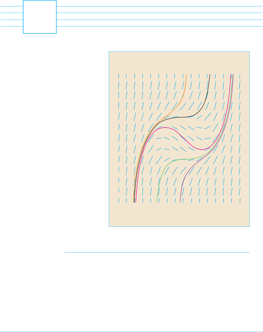
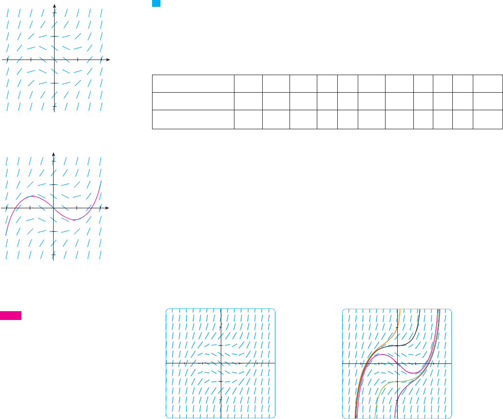
EXAMPLE 1

(a) Sketch the direction ﬁeld for the differential equation .

(b) Use part (a) to sketch the solution curve that passes through the origin.

SOLUTION

(a) We start by computing the slope at several points in the following chart:

Now we draw short line segments with these slopes at these points. The result is the

direction ﬁeld shown in Figure 5.

(b) We start at the origin and move to the right in the direction of the line segment

(which has slope ). We continue to draw the solution curve so that it moves parallel

to the nearby line segments. The resulting solution curve is shown in Figure 6. Returning

to the origin, we draw the solution curve to the left as well. M

The more line segments we draw in a direction ﬁeld, the clearer the picture becomes.

Of course, it’s tedious to compute slopes and draw line segments for a huge number of

points by hand, but computers are well suited for this task. Figure 7 shows a more detailed,

computer-drawn direction ﬁeld for the differential equation in Example 1. It enables us to

draw, with reasonable accuracy, the solution curves shown in Figure 8 with -intercepts

, , , , and .

F I G U R E 7

_3 3

F I G U R E 8

_3 3

210#1#2

y" ! x

% y

# 1

!x, y"F!x, y"

F!x, y"!x, y"

yxF!x, y"

y" ! F!x, y"

!0, 1"

SECTION 10.2 DIRECTION FIELDS AND EULER’S METHOD

|| ||

609

x #2 #1 0 1 2 #2 #1 0 1 2 . . .

y 0 0 0 0 0 1 1 1 1 1 . . .

3 0 #1 0 3 4 1 0 1 4 . . .y" ! x

% y

# 1

1_1_2

-1

F I G U R E 5

Module 10.2A shows direction

ﬁelds and solution curves for a variety of

differential equations.

TE C

1 2_1_2

-1

F I G U R E 6

Now let’s see how direction ﬁelds give insight into physical situations. The simple elec-

tric circuit shown in Figure 9 contains an electromotive force (usually a battery or gener-

ator) that produces a voltage of volts (V) and a current of amperes (A) at time t.

The circuit also contains a resistor with a resistance of R ohms ( ) and an inductor with

an inductance of L henries (H).

Ohm’s Law gives the drop in voltage due to the resistor as RI. The voltage drop due to

the inductor is . One of Kirchhoff’s laws says that the sum of the voltage drops is

equal to the supplied voltage . Thus we have

which is a ﬁrst-order differential equation that models the current at time .

EXAMPLE 2 Suppose that in the simple circuit of Figure 9 the resistance is , the

inductance is 4 H, and a battery gives a constant voltage of 60 V.

(a) Draw a direction ﬁeld for Equation 1 with these values.

(b) What can you say about the limiting value of the current?

(d) If the switch is closed when so the current starts with , use the direc-

tion ﬁeld to sketch the solution curve.

SOLUTION

(a) If we put , , and in Equation 1, we get

The direction ﬁeld for this differential equation is shown in Figure 10.

(b) It appears from the direction ﬁeld that all solutions approach the value 5 A, that is,

can verify this directly from the differential equation . If , then

the left side is and the right side is .15 # 3!5" ! 0dI#dt ! 0

I!t" ! 5dI#dt ! 15 # 3I

I!t" ! 5

lim

I!t" ! 5

F I G U R E 1 0

0 t

2 3

! 15 # 3Ior4

% 12I ! 60

E!t" ! 60R ! 12L ! 4

I!0" ! 0t ! 0

12 +

% RI ! E!t"

E!t"

L!dI#dt"

I!t"E!t"

610

|| ||

CHAPTER 10 DIFFERENTIAL EQUATIONS

switch

F I G U R E 9

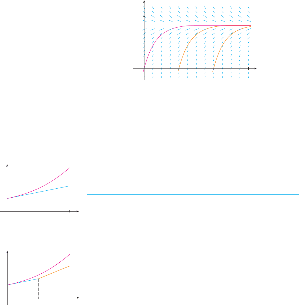
(d) We use the direction ﬁeld to sketch the solution curve that passes through , as

shown in red in Figure 11.

Notice from Figure 10 that the line segments along any horizontal line are parallel. That

is because the independent variable t does not occur on the right side of the equation

. In general, a differential equation of the form

in which the independent variable is missing from the right side, is called autonomous.

For such an equation, the slopes corresponding to two different points with the same

y-coordinate must be equal. This means that if we know one solution to an autonomous

differential equation, then we can obtain inﬁnitely many others just by shifting the graph

of the known solution to the right or left. In Figure 11 we have shown the solutions

that result from shifting the solution curve of Example 2 one and two time units (namely,

seconds) to the right. They correspond to closing the switch when or .

EULER’S METHOD

The basic idea behind direction ﬁelds can be used to ﬁnd numerical approximations to

solutions of differential equations. We illustrate the method on the initial-value problem

that we used to introduce direction ﬁelds:

The differential equation tells us that , so the solution curve has slope

1 at the point . As a ﬁrst approximation to the solution we could use the linear approx-

imation . In other words, we could use the tangent line at as a rough

approximation to the solution curve (see Figure 12).

Euler’s idea was to improve on this approximation by proceeding only a short distance

along this tangent line and then making a midcourse correction by changing direction as

indicated by the direction ﬁeld. Figure 13 shows what happens if we start out along the

tangent line but stop when . (This horizontal distance traveled is called the step

size.) Since , we have and we take as the starting point

for a new line segment. The differential equation tells us that , so

we use the linear function

y ! 1.5 % 2!x # 0.5" ! 2x % 0.5

y"!0.5" ! 0.5 % 1.5 ! 2

!0.5, 1.5"y!0.5" $ 1.5L!0.5" ! 1.5

x ! 0.5

!0, 1"L!x" ! x % 1

!0, 1"

y"!0" ! 0 % 1 ! 1

y!0" ! 1y" ! x % y

t ! 2t ! 1

y" ! f !y

I" ! 15 # 3I

F I G U R E 1 1

0 t

2 3

!0, 0"

SECTION 10.2 DIRECTION FIELDS AND EULER’S METHOD

|| ||

611

y=L(x)

solution curve

F I G U R E 1 2

First Euler approximation

0.5

1.5

F I G U R E 1 3

Euler approximation with step size 0.5