Stewart J. Calculus

Подождите немного. Документ загружается.

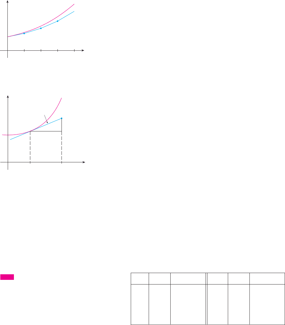
as an approximation to the solution for (the orange segment in Figure 13). If we

decrease the step size from to , we get the better Euler approximation shown in

Figure 14.

In general, Euler’s method says to start at the point given by the initial value and pro-

ceed in the direction indicated by the direction ﬁeld. Stop after a short time, look at the

slope at the new location, and proceed in that direction. Keep stopping and changing direc-

tion according to the direction ﬁeld. Euler’s method does not produce the exact solution to

an initial-value problem—it gives approximations. But by decreasing the step size (and

therefore increasing the number of midcourse corrections), we obtain successively better

approximations to the exact solution. (Compare Figures 12, 13, and 14.)

For the general ﬁrst-order initial-value problem , , our aim is to

ﬁnd approximate values for the solution at equally spaced numbers , ,

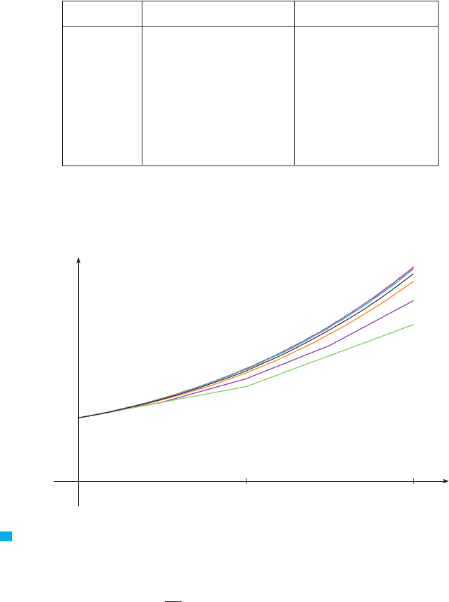
, . . . , where is the step size. The differential equation tells us that the slope

at is , so Figure 15 shows that the approximate value of the solution

when is

Similarly,

In general,

EXAMPLE 3 Use Euler’s method with step size to construct a table of approximate

values for the solution of the initial-value problem

SOLUTION We are given that , , , and . So we have

This means that if is the exact solution, then .

Proceeding with similar calculations, we get the values in the table:

For a more accurate table of values in Example 3 we could decrease the step size. But

for a large number of small steps the amount of computation is considerable and so we

need to program a calculator or computer to carry out these calculations. The following

table shows the results of applying Euler’s method with decreasing step size to the initial-

value problem of Example 3.

y!0.3" # 1.362y!x"

! y

! hF!x

, y

" ! 1.22 ! 0.1!0.2 ! 1.22" ! 1.362

! y

! hF!x

, y

" ! 1.1 ! 0.1!0.1 ! 1.1" ! 1.22

! y

! hF!x

, y

" ! 1 ! 0.1!0 ! 1" ! 1.1

F!x, y" ! x ! yy

! 1x

! 0h ! 0.1

y!0" ! 1y" ! x ! y

0.1

! y

n#1

! hF!x

n#1

, y

n#1

! y

! hF!x

, y

! y

! hF!x

, y

x ! x

y" ! F!x

, y

"!x

, y

! x

! h

! x

! hx

y!x

" ! y

y" ! F!x, y"

0.250.5

x $ 0.5

612

|| ||

CHAPTER 10 DIFFERENTIAL EQUATIONS

n n

1 0.1 1.100000 6 0.6 1.943122

0.2 1.220000 7 0.7 2.197434

3 0.3 1.362000 8 0.8 2.487178

4 0.4 1.528200 9 0.9 2.815895

5 0.5 1.721020 10 1.0 3.187485

⁄x¸

y¸

h F(x¸,y¸)

(⁄,›)

slope=F(x¸,y¸)

F I G U R E 1 5

0.25

F I G U R E 1 4

Euler approximation with step size 0.25

Module 10.2B shows how Euler’s

method works numerically and visually

for a variety of differential equations and

step sizes.

TE C

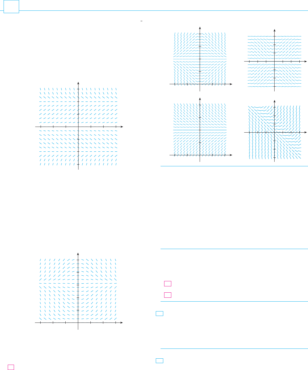
Notice that the Euler estimates in the table seem to be approaching limits, namely, the

true values of and . Figure 16 shows graphs of the Euler approximations with

step sizes 0.5, 0.25, 0.1, 0.05, 0.02, 0.01, and 0.005. They are approaching the exact solu-

tion curve as the step size h approaches 0.

EXAMPLE 4 In Example 2 we discussed a simple electric circuit with resistance

, inductance 4 H, and a battery with voltage 60 V. If the switch is closed when

, we modeled the current I at time t by the initial-value problem

Estimate the current in the circuit half a second after the switch is closed.

SOLUTION We use Euler’s method with , and step size

second:

So the current after 0.5 seconds is

MI!0.5" # 4.16 A

! 3.7995 ! 0.1!15 # 3 ! 3.7995" ! 4.15965

! 3.285 ! 0.1!15 # 3 ! 3.285" ! 3.7995

! 2.55 ! 0.1!15 # 3 ! 2.55" ! 3.285

! 1.5 ! 0.1!15 # 3 ! 1.5" ! 2.55

! 0 ! 0.1!15 # 3 ! 0" ! 1.5

h ! 0.1

F!t, I" ! 15 # 3I, t

! 0, I

! 0

I!0" ! 0

! 15 # 3I

t ! 0

12 %

0 x

0.5 1

F I G U R E 1 6

Euler approximations

approaching the exact solution

y!1"y!0.5"

SECTION 10.2 DIRECTION FIELDS AND EULER’S METHOD

|| ||

613

Step size Euler estimate of Euler estimate of

0.500 1.500000 2.500000

0.250

1.625000 2.882813

0.100 1.721020 3.187485

0.050 1.757789 3.306595

0.020 1.781212 3.383176

0.010 1.789264 3.409628

0.005 1.793337 3.423034

0.001 1.796619 3.433848

y!1"y!0.5"

N Computer software packages that produce

numerical approximations to solutions of

differential equations use methods that are

reﬁnements of Euler’s method. Although Euler’s

method is simple and not as accurate, it is the

basic idea on which the more accurate methods

are based.

614

|| ||

CHAPTER 10 DIFFERENTIAL EQUATIONS

5. 6.

7. Use the direction ﬁeld labeled II (above) to sketch the graphs

of the solutions that satisfy the given initial conditions.

(a) (b) (c)

8. Use the direction ﬁeld labeled IV (above) to sketch the graphs

of the solutions that satisfy the given initial conditions.

(a) (b) (c)

9–10 Sketch a direction ﬁeld for the differential equation. Then

use it to sketch three solution curves.

9. 10.

11–14 Sketch the direction ﬁeld of the differential equation.

Then use it to sketch a solution curve that passes through the

given point.

12. ,

14. ,

15–16 Use a computer algebra system to draw a direction ﬁeld

for the given differential equation. Get a printout and sketch on it

the solution curve that passes through . Then use the CAS to

draw the solution curve and compare it with your sketch.

15. 16.

17. Use a computer algebra system to draw a direction ﬁeld for

the differential equation . Get a printout and y" ! y

# 4y

CAS

y" ! x!y

# 4"y" ! x

sin y

!0, 1"

CAS

!1, 0"y" ! x # xy!0, 1"y" ! y ! x y

13.

!0, 0"y" ! 1 # x y!1, 0"y" ! y # 2x

11.

y" ! x

# y

y" ! 1 ! y

y!0" ! 1y!0" ! 0y!0" ! #1

y!0" ! #1y!0" ! 2y!0" ! 1

2_2

I II

III IV

y" ! sin x sin yy" ! x ! y # 1

1. A direction ﬁeld for the differential equation

is shown.

(a) Sketch the graphs of the solutions that satisfy the given

initial conditions.

(i) (ii)

(iii) (iv)

(b) Find all the equilibrium solutions.

2. A direction ﬁeld for the differential equation is

shown.

(a) Sketch the graphs of the solutions that satisfy the given

initial conditions.

(i) (ii) (iii)

(iv) (v)

(b) Find all the equilibrium solutions.

3–6 Match the differential equation with its direction ﬁeld

(labeled I–IV). Give reasons for your answer.

4. y" ! x!2 # y"y" ! 2 # y

3_3

1 2_1_2

y!0" ! 5y!0" ! 4

y!0" !

y!0" ! 2y!0" ! 1

y" ! x sin y

3_3

1 2_1_2

y!0" ! 3y!0" ! #3

y!0" ! #1y!0" ! 1

y" ! y

(

1 #

)

E X E R C I S E S

10.2

22. Use Euler’s method with step size to estimate , where

is the solution of the initial-value problem ,

Use Euler’s method with step size to estimate ,

where is the solution of the initial-value problem

, .

24. (a) Use Euler’s method with step size to estimate ,

where is the solution of the initial-value problem

, .

(b) Repeat part (a) with step size .

;

25. (a) Program a calculator or computer to use Euler’s method

to compute , where is the solution of the initial-

value problem

(i) (ii)

(iii) (iv)

(b) Verify that is the exact solution of the

differential equation.

with the step sizes in part (a). What happens to the error

when the step size is divided by 10?

26. (a) Program your computer algebra system, using Euler’s

method with step size 0.01, to calculate , where

is the solution of the initial-value problem

(b) Check your work by using the CAS to draw the solution

curve.

27. The ﬁgure shows a circuit containing an electromotive force,

a capacitor with a capacitance of farads (F), and a resistor

with a resistance of ohms ( ). The voltage drop across the

capacitor is , where is the charge (in coulombs), so in

this case Kirchhoff’s Law gives

But , so we have

Suppose the resistance is , the capacitance is F, and a

battery gives a constant voltage of 60 V.

(a) Draw a direction ﬁeld for this differential equation.

(b) What is the limiting value of the charge?

0.05%5

Q ! E!t"

I ! dQ$dt

RI !

! E!t"

QQ$C

y!0" ! 1y" ! x

# y

yy!2"

CAS

y!1"

y ! 2 ! e

h ! 0.001h ! 0.01

h ! 0.1h ! 1

y!0" ! 3

! 3x

y ! 6x

y!x"y!1"

0.1

y!1" ! 0y" ! x # xy

y!x"

y!1.4"0.2

y!0" ! 1y" ! y ! xy

y!x"

y!0.5"0.1

23.

y!0" ! 0

y" ! 1 # x yy!x"

y!1"0.2

sketch on it solutions that satisfy the initial condition

for various values of . For what values of does

exist? What are the possible values for this limit?

Make a rough sketch of a direction ﬁeld for the autonomous

differential equation , where the graph of is as

shown. How does the limiting behavior of solutions depend

on the value of ?

(a) Use Euler’s method with each of the following step sizes

to estimate the value of , where is the solution of

the initial-value problem .

(i) (ii) (iii)

(b) We know that the exact solution of the initial-value

problem in part (a) is . Draw, as accurately as you

can, the graph of , together with the

Euler approximations using the step sizes in part (a).

(Your sketches should resemble Figures 12, 13, and 14.)

Use your sketches to decide whether your estimates in

part (a) are underestimates or overestimates.

the exact value and the approximate value. Find the errors

made in part (a) in using Euler’s method to estimate the

true value of , namely . What happens to the

error each time the step size is halved?

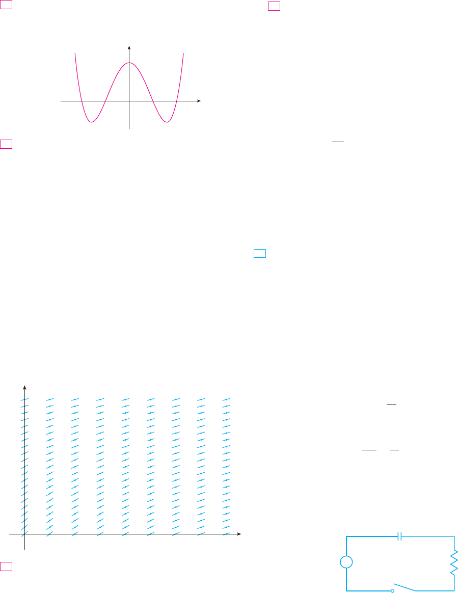
20. A direction ﬁeld for a differential equation is shown. Draw,

with a ruler, the graphs of the Euler approximations to the

solution curve that passes through the origin. Use step sizes

and . Will the Euler estimates be under-

estimates or overestimates? Explain.

Use Euler’s method with step size to compute the approx-

imate -values of the solution of the initial-

value problem , .y!1" ! 0y" ! y # 2x

, y

, and y

0.5

21.

1 2

h ! 0.5h ! 1

0.4

y!0.4"

y ! e

, 0 ' x ' 0.4

y ! e

h ! 0.1h ! 0.2h ! 0.4

y" ! y, y!0" ! 1

yy!0.4"

19.

0 y

_1_2

f(y)

y!0"

fy" ! f !y"

18.

lim

(

y!t"

ccy!0" ! c

SECTION 10.2 DIRECTION FILEDS AND EULER’S METHOD

|| ||

615

at a rate of per minute when its temperature is .

(a) What does the differential equation become in this case?

(b) Sketch a direction ﬁeld and use it to sketch the solution

curve for the initial-value problem. What is the limiting

value of the temperature?

estimate the temperature of the coffee after 10 minutes.

h ! 2

70)C1)C

(d) If the initial charge is , use the direction ﬁeld to

sketch the solution curve.

(e) If the initial charge is , use Euler’s method with

step size 0.1 to estimate the charge after half a second.

28. In Exercise 14 in Section 10.1 we considered a cup of cof-

fee in a room. Suppose it is known that the coffee cools 20)C

95)C

Q!0" ! 0 C

616

|| ||

CHAPTER 10 DIFFERENTIAL EQUATIONS

SEPARABLE EQUATIONS

We have looked at ﬁrst-order differential equations from a geometric point of view (direc-

tion ﬁelds) and from a numerical point of view (Euler’s method). What about the symbolic

point of view? It would be nice to have an explicit formula for a solution of a differential

equation. Unfortunately, that is not always possible. But in this section we examine a cer-

tain type of differential equation that can be solved explicitly.

A separable equation is a ﬁrst-order differential equation in which the expression for

can be factored as a function of x times a function of y. In other words, it can be

written in the form

The name separable comes from the fact that the expression on the right side can be “sep-

arated” into a function of and a function of . Equivalently, if , we could write

where . To solve this equation we rewrite it in the differential form

so that all ’s are on one side of the equation and all ’s are on the other side. Then we inte-

grate both sides of the equation:

Equation 2 deﬁnes implicitly as a function of . In some cases we may be able to solve

for in terms of .

We use the Chain Rule to justify this procedure: If and satisfy (2), then

and

Thus Equation 1 is satisﬁed.

h!y"

! t!x"

h!y" dy

! t!x"

h!y" dy

t!x" dx

h!y" dy !

t!x" dx

h!y" dy ! t!x" dx

h!y" ! 1$f !y"

t!x"

h!y"

f !y" " 0yx

! t!x"f !y"

dy$dx

10.3

N The technique for solving separable differen-

tial equations was ﬁrst used by James Bernoulli

(in 1690) in solving a problem about pendulums

and by Leibniz (in a letter to Huygens in 1691).

John Bernoulli explained the general method in a

paper published in 1694.

EXAMPLE 1

(a) Solve the differential equation .

(b) Find the solution of this equation that satisﬁes the initial condition .

SOLUTION

(a) We write the equation in terms of differentials and integrate both sides:

where is an arbitrary constant. (We could have used a constant on the left side and

another constant on the right side. But then we could combine these constants by

writing .)

Solving for , we get

We could leave the solution like this or we could write it in the form

where . (Since is an arbitrary constant, so is .)

(b) If we put in the general solution in part (a), we get . To satisfy the

initial condition , we must have and so .

Thus the solution of the initial-value problem is

EXAMPLE 2 Solve the differential equation .

SOLUTION Writing the equation in differential form and integrating both sides, we have

where is a constant. Equation 3 gives the general solution implicitly. In this case it’s

impossible to solve the equation to express explicitly as a function of . M

EXAMPLE 3 Solve the equation .

SOLUTION First we rewrite the equation using Leibniz notation:

! x

y" ! x

! sin y ! 2x

! C

!2y ! cos y"dy !

!2y ! cos y"dy ! 6x

2y ! cos y

y !

! 8

K ! 8

! 2y!0" ! 2

y!0" !

x ! 0

KCK ! 3C

y !

! K

y !

! 3C

C ! C

# C

! C

dy !

dy ! x

y!0" ! 2

SECTION 10.3 SEPARABLE EQUATIONS

|| ||

617

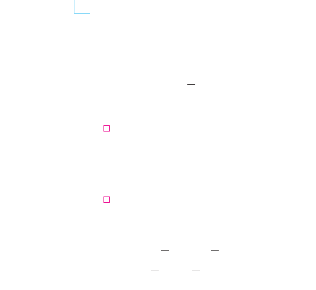
N Figure 1 shows graphs of several members

of the family of solutions of the differential

equation in Example 1. The solution of the initial-

value problem in part (b) is shown in red.

_3 3

F I G U R E 1

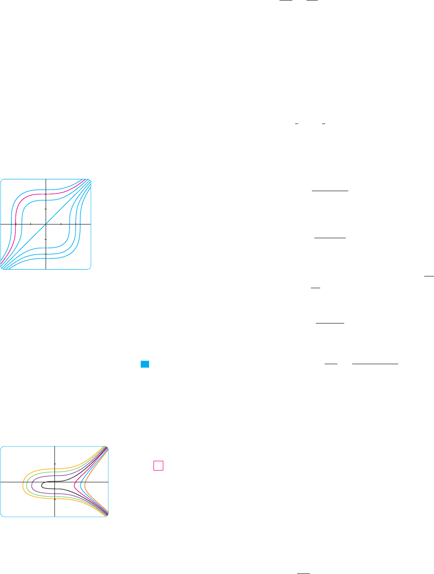
N Some computer algebra systems can plot

curves deﬁned by implicit equations. Figure 2

shows the graphs of several members of the

family of solutions of the differential equation

in Example 2. As we look at the curves from left

to right, the values of are , , , , , ,

and .#3

#2#10123C

_2 2

F I G U R E 2

If , we can rewrite it in differential notation and integrate:

This equation deﬁnes implicitly as a function of . But in this case we can solve

explicitly for as follows:

We can easily verify that the function is also a solution of the given differential

equation. So we can write the general solution in the form

where is an arbitrary constant ( , or , or ). M

EXAMPLE 4 In Section 10.2 we modeled the current in the electric circuit shown

in Figure 5 by the differential equation

Find an expression for the current in a circuit where the resistance is , the induc-

tance is 4 H, a battery gives a constant voltage of 60 V, and the switch is turned on when

. What is the limiting value of the current?

SOLUTION With L ! 4, R ! 12, and , the equation becomes

! 15 # 3I 4

! 12I ! 60

E!t" ! 60

t ! 0

12 %

! RI ! E!t"

I!t"

_2 2

F I G U R E 4

F I G U R E 3

1 2_1_2

A ! 0A ! #e

A ! e

y ! Ae

y ! 0

y ! *e

! e

$3"!C

! e

! C

! x

dx y " 0

y " 0

618

|| ||

CHAPTER 10 DIFFERENTIAL EQUATIONS

N If a solution is a function that satisﬁes

for some , it follows from a

uniqueness theorem for solutions of differential

equations that for all .xy!x" " 0

xy!x" " 0

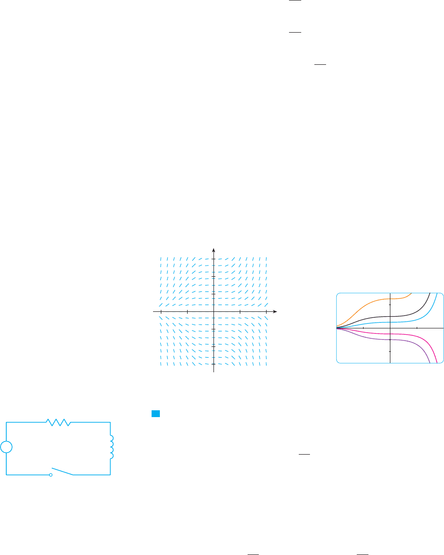
N Figure 3 shows a direction ﬁeld for the differ-

ential equation in Example 3. Compare it with

Figure 4, in which we use the equation

to graph solutions for several values

of . If you use the direction ﬁeld to sketch

solution curves with -intercepts , , , ,

and , they will resemble the curves in

Figure 4.

#1125y

y ! Ae

switch

F I G U R E 5

and the initial-value problem is

We recognize this equation as being separable, and we solve it as follows:

Since , we have , so A ! 15 and the solution is

The limiting current, in amperes, is

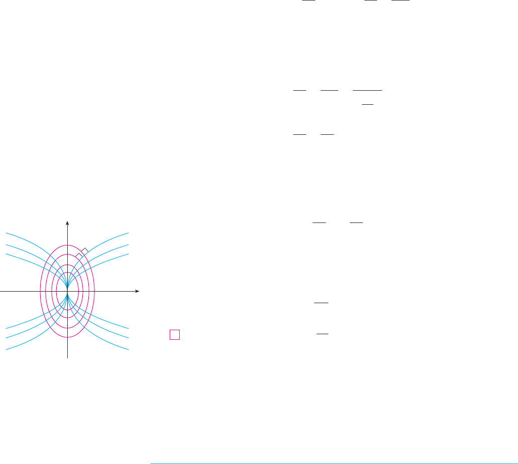
ORTHOGONAL TRA JECTORIES

An orthogonal trajectory of a family of curves is a curve that intersects each curve of the

family orthogonally, that is, at right angles (see Figure 7). For instance, each member of

the family of straight lines through the origin is an orthogonal trajectory of the

family of concentric circles with center the origin (see Figure 8). We say that

the two families are orthogonal trajectories of each other.

EXAMPLE 5 Find the orthogonal trajectories of the family of curves , where

is an arbitrary constant.

SOLUTION The curves form a family of parabolas whose axis of symmetry is

the -axis. The ﬁrst step is to ﬁnd a single differential equation that is satisﬁed by all x

x ! ky

F I G U R E 8

orthogonal

trajectory

F I G U R E 7

! y

! r

y ! mx

! 5 # 0 ! 5 lim

(

I!t" ! lim

(

!5 # 5e

#3t

" ! 5 # 5 lim

(

#3t

I!t" ! 5 # 5e

#3t

5 #

A ! 0I!0" ! 0

I ! 5 #

#3t

15 # 3I ! *e

#3C

#3t

! Ae

#3t

15 # 3I

! e

#3!t!C"

15 # 3I

! t ! C

!15 # 3I " 0"

15 # 3I

I!0" ! 0

! 15 # 3I

SECTION 10.3 SEPARABLE EQUATIONS

|| ||

619

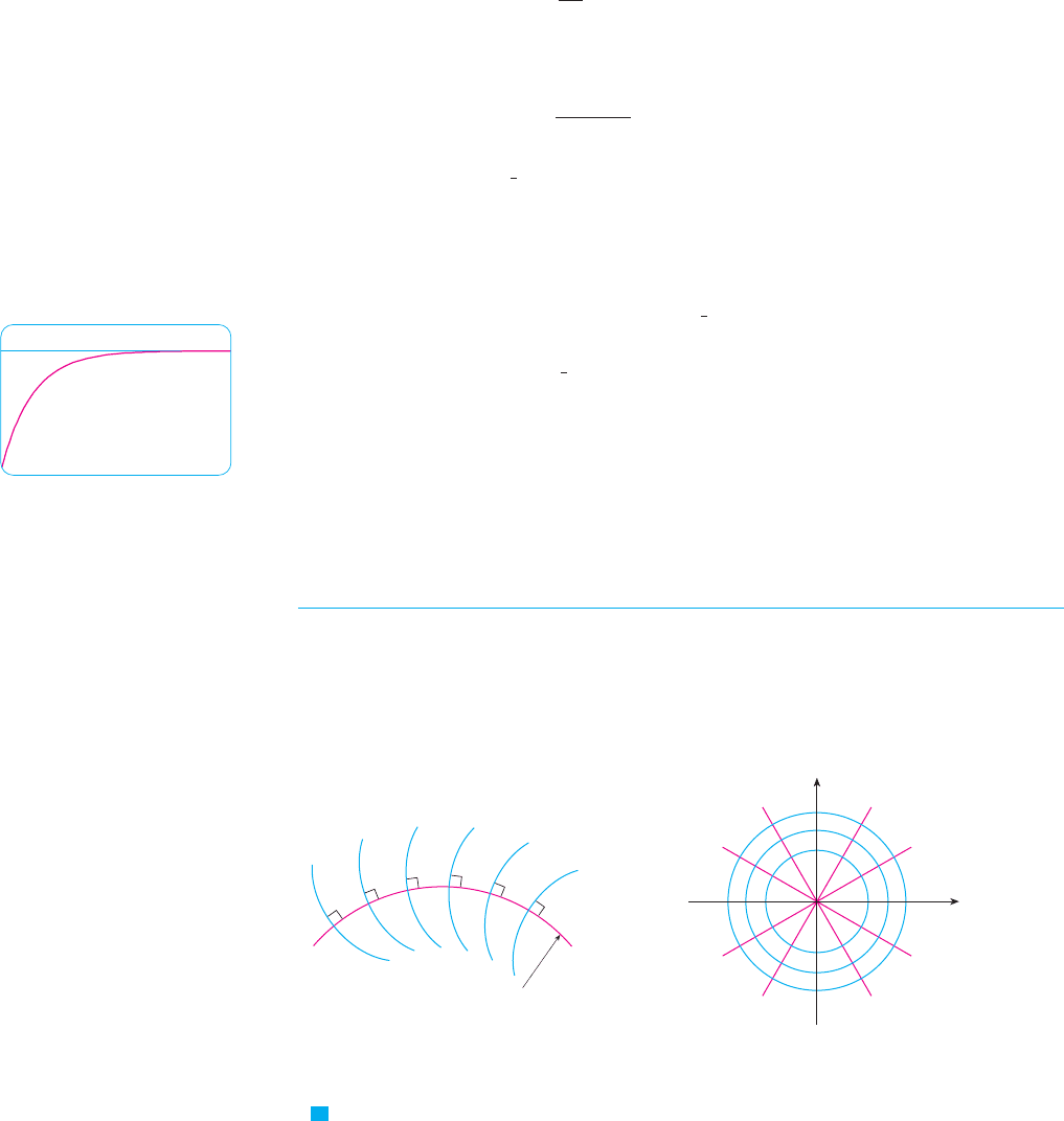
N Figure 6 shows how the solution in Example 4

(the current) approaches its limiting value. Com-

parison with Figure 11 in Section 10.2 shows

that we were able to draw a fairly accurate

solution curve from the direction ﬁeld.

2.5

y=5

F I G U R E 6

members of the family. If we differentiate , we get

This differential equation depends on , but we need an equation that is valid for all

values of simultaneously. To eliminate we note that, from the equation of the given

general parabola , we have and so the differential equation can be

written as

This means that the slope of the tangent line at any point on one of the parabolas is

. On an orthogonal trajectory the slope of the tangent line must be the nega-

tive reciprocal of this slope. Therefore the orthogonal trajectories must satisfy the differ-

ential equation

This differential equation is separable, and we solve it as follows:

where is an arbitrary positive constant. Thus the orthogonal trajectories are the family

of ellipses given by Equation 4 and sketched in Figure 9.

Orthogonal trajectories occur in various branches of physics. For example, in an elec-

trostatic ﬁeld the lines of force are orthogonal to the lines of constant potential. Also,

the streamlines in aerodynamics are orthogonal trajectories of the velocity-equipotential

curves.

MIXING PROBLEMS

A typical mixing problem involves a tank of ﬁxed capacity ﬁlled with a thoroughly mixed

solution of some substance, such as salt. A solution of a given concentration enters the tank

at a ﬁxed rate and the mixture, thoroughly stirred, leaves at a ﬁxed rate, which may differ

from the entering rate. If denotes the amount of substance in the tank at time t, then

is the rate at which the substance is being added minus the rate at which it is being

removed. The mathematical description of this situation often leads to a ﬁrst-order sepa-

rable differential equation. We can use the same type of reasoning to model a variety of

phenomena: chemical reactions, discharge of pollutants into a lake, injection of a drug into

the bloodstream.

y"!t"

y!t"

! C

! #x

! C

y dy ! #

2x dx

! #

y" ! y$!2x"

!x, y"

2ky

k ! x$y

x ! ky

2ky

or1 ! 2ky

x ! ky

620

|| ||

CHAPTER 10 DIFFERENTIAL EQUATIONS

F I G U R E 9

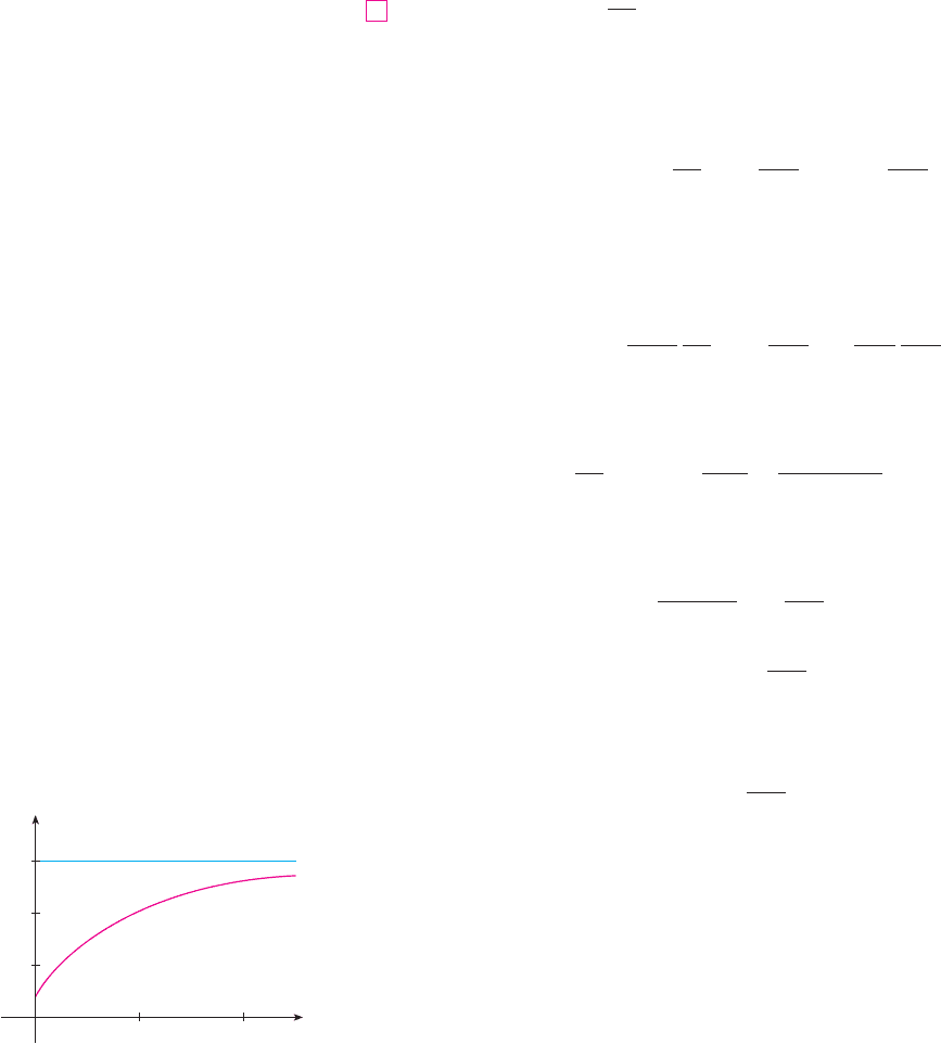
EXAMPLE 6 A tank contains 20 kg of salt dissolved in 5000 L of water. Brine that con-

tains 0.03 kg of salt per liter of water enters the tank at a rate of 25 L$min. The solution

is kept thoroughly mixed and drains from the tank at the same rate. How much salt

remains in the tank after half an hour?

SOLUTION Let be the amount of salt (in kilograms) after minutes. We are given that

and we want to ﬁnd . We do this by ﬁnding a differential equation satis-

ﬁed by . Note that is the rate of change of the amount of salt, so

where (rate in) is the rate at which salt enters the tank and (rate out) is the rate at which

salt leaves the tank. We have

The tank always contains 5000 L of liquid, so the concentration at time is

(measured in kilograms per liter). Since the brine ﬂows out at a rate of 25 L$min, we

have

Thus, from Equation 5, we get

Solving this separable differential equation, we obtain

Since , we have , so

Therefore

Since is continuous and and the right side is never 0, we deduce that

is always positive. Thus and so

The amount of salt after 30 min is

y!30" ! 150 # 130e

#30$200

# 38.1 kg

y!t" ! 150 # 130e

#t$200

150 # y

! 150 # y150 # y!t"

y!0" ! 20y!t"

150 # y

! 130e

#t$200

#ln

150 # y

200

# ln 130

#ln 130 ! Cy!0" ! 20

#ln

150 # y

200

! C

150 # y

200

! 0.75 #

y!t"

200

150 # y!t"

200

rate out !

y!t"

5000

min

y!t"

200

min

y!t"$5000t

rate in !

0.03

min

! 0.75

min

! !rate in" # !rate out"

dy$dty!t"

y!30"y!0" ! 20

ty!t"

SECTION 10.3 SEPARABLE EQUATIONS

|| ||

621

N Figure 10 shows the graph of the function

of Example 6. Notice that, as time goes by, the

amount of salt approaches 150 kg.

y!t"

200 400

100

150

F I G U R E 1 0