Sundararaja D. The Discrete Fourier Transform. Theory, Algorithms and Applications
Подождите немного. Документ загружается.

204
Two-Dimensional Discrete Fourier Transform
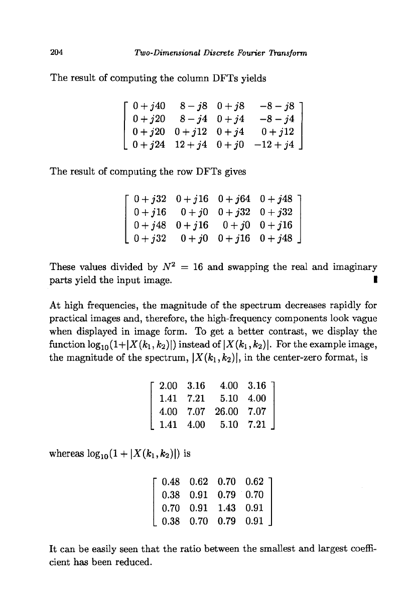
The result of computing the column DFTs yields
0 + j'40
0+J20
0+J20
0+J24
8-j8
8-j4
0+jU
12 + J4
O+j/8
0+j'4
0+;?4
0 + j0
-8 - j8
-8 - j4
0 + J12
-12 + J4
The result of computing the row DFTs gives
0+J32 0+J16
0+J16 0 + j0
0+j'48 0+J16
O
+
j'32
0 + j0
0 + j64 0 + j48
0 + j32 0 + j32
0 + ;0 0 + jl6
0 +
j"16
0 + j48
These values divided by iV
2
=
parts yield the input image.
16 and swapping the real and imaginary
At high frequencies, the magnitude of the spectrum decreases rapidly for
practical images and, therefore, the high-frequency components look vague
when displayed in image form. To get a better contrast, we display the
function log
10
(l+|X(A;i, /t
2
)|) instead of \X(ki,k
2
)\. For the example image,
the magnitude of the spectrum, |X(fci,A;2)|, in the center-zero format, is
2.00 3.16 4.00 3.16
1.41 7.21 5.10 4.00
4.00 7.07 26.00 7.07
1.41 4.00 5.10 7.21
whereas log
10
(l + |X(fci,fc
2
)|) is
0.48 0.62 0.70 0.62
0.38 0.91 0.79 0.70
0.70 0.91 1.43 0.91
0.38 0.70 0.79 0.91
It can be easily seen that the ratio between the smallest and largest coeffi-
cient has been reduced.
Properties of the 2-D DFT 205
10.4 Properties of the 2-D DFT
Linearity
The DFT of a linear combination of a set of discrete images is equal to
the same linear combination of the individual DFTs of the images. Let
xi{ni,n
2
)
<$
Xi(ki,k
2
) and £
2
(ni,n
2
)
<$
X
2
(ki,k
2
).
Then,
axi(ni,ri2) + bx2(ni,n,2) O a-X"i(fci,fc
2
) +
6X2(^1,
fc
2
)
where a and 6 are real or complex constants. It is assumed that the images
have same dimensions. If it is not so, sufficient zero padding must be done.
Linearity holds in both the spatial time- and frequency-domains.
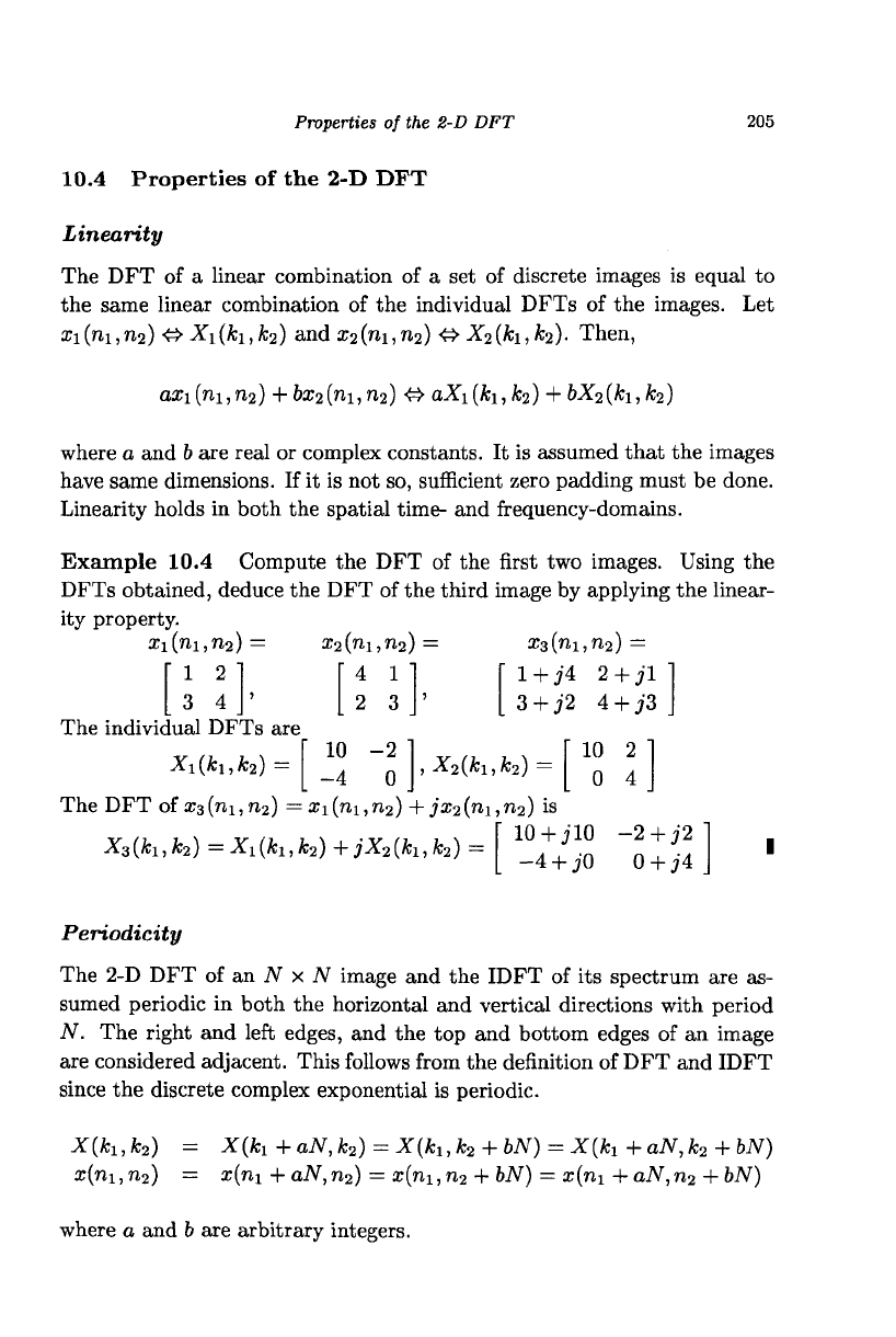
Example 10.4 Compute the DFT of the first two images. Using the
DFTs obtained, deduce the DFT of the third image by applying the linear-
ity property.
X\
The indivic
(ni,n
2
)
12'
3 4
lual DF
Xi(*iJ
=
x^
Is are
c
2
) =
1
(ni,n
2
)
"41'
2 3
3 -2 "
4 0
1
,X
2
(k
u
x
3
(ni,n
2
) =
' 1+J4 2 + jl'
. 3 + J
k
2
) =
2 4 + j'i
10 2'
0 4
1
The DFT of X3(ni,n
2
) = xi(ni,n
2
) + jx
2
(ni,n
2
) is
*
3
(*i,
fo)=Ji :i(h,)
c
2
)-
rjX
2
(k
l.fa) =
" io+.
-4 +
;'10 -2
JO 0
7'2"
74.
Periodicity
The 2-D DFT of an N x N image and the IDFT of its spectrum are as-
sumed periodic in both the horizontal and vertical directions with period
N. The right and left edges, and the top and bottom edges of an image
are considered adjacent. This follows from the definition of DFT and IDFT
since the discrete complex exponential is periodic.
-X"(*i,*a) = X(k
1
+aN,k
2
) = X(ki,k
2
+ bN) = X{k
1
+aN,k
2
+bN)
x(ni,n
2
) = x(ni+aN,n
2
) = x(ni,n
2
+ bN) = x(n!+aN,n
2
+bN)
where a and b are arbitrary integers.
206
Two-Dimensional Discrete Fourier Transform
Spatial circular shift of an image
The shift of an image can be carried out in two steps: (i) shift each row to
the right or left as required and (ii) shift each column upwards or down-
wards as required. Let 2(711,712) •£> X(ki,k
2
). Then, x{n\
—
I,n
2
—
m) 4^
X(k
u
k
2
)W^
ll+k2m)
.
As in the case of 1-D DFT, the spatial shift of
#(711,712) does not affect the magnitude of the spectrum but only changes
the phase.
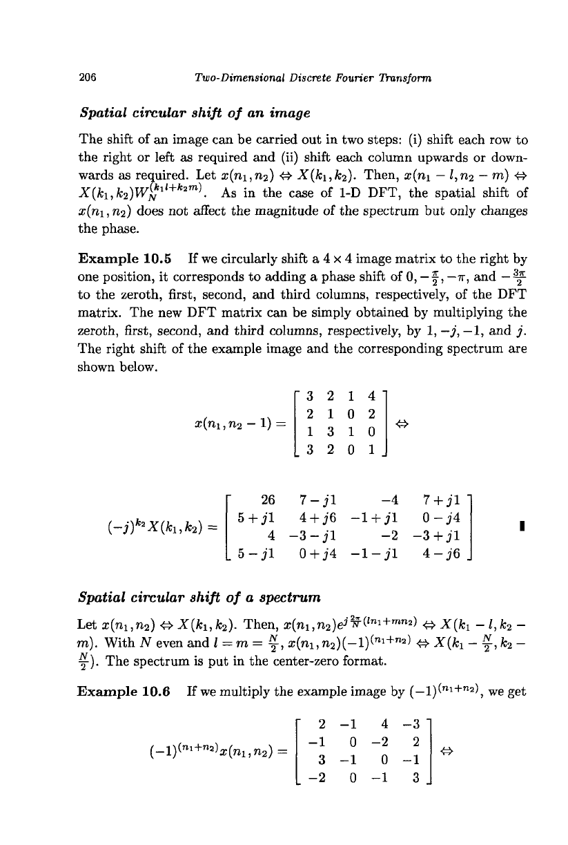
Example 10.5 If we circularly shift a 4 x 4 image matrix to the right by
one position, it corresponds to adding a phase shift of 0,
—
f, —
n,
and
—
^
L
to the zeroth, first, second, and third columns, respectively, of the DFT
matrix. The new DFT matrix can be simply obtained by multiplying the
zeroth, first, second, and third columns, respectively, by
1,—
j,
—
1,
and j.
The right shift of the example image and the corresponding spectrum are
shown below.
2j(7ii,n
2
- 1) =
3 2 14
2 10 2
13 10
3 2 0 1
<$
(-j)
k
*X(k
u
k
2
) =
26
5 + jl
4
5-jl
7-jl
4 + j6
-3-jl
0+j4
-4
-1 + j'l
-2
-1-jl
7 + jl
0-J4
-3 + jl
4-j6
Spatial circular shift of a spectrum
Let x(n
1
,n
2
)&X(k
u
k
2
). Then, x(n
u
n
2
)e
j
^
ln
^
+mn
^ &X{h -l,k
2
-
m).
With N even and I = m = f, x(ni,n
2
)(-l)("
1+
"
2
)
<S>
X(h - f, k
2
-
y).
The spectrum is put in the center-zero format.
Example 10.6 If we multiply the example image
by (-l)("i+"=), we get
{-l)(
ni+n
^x(n
u
n
2
) =
2
1
3
2
-1
0
-1
0
4
-2
0
-1
-3
2
-1
3
4>
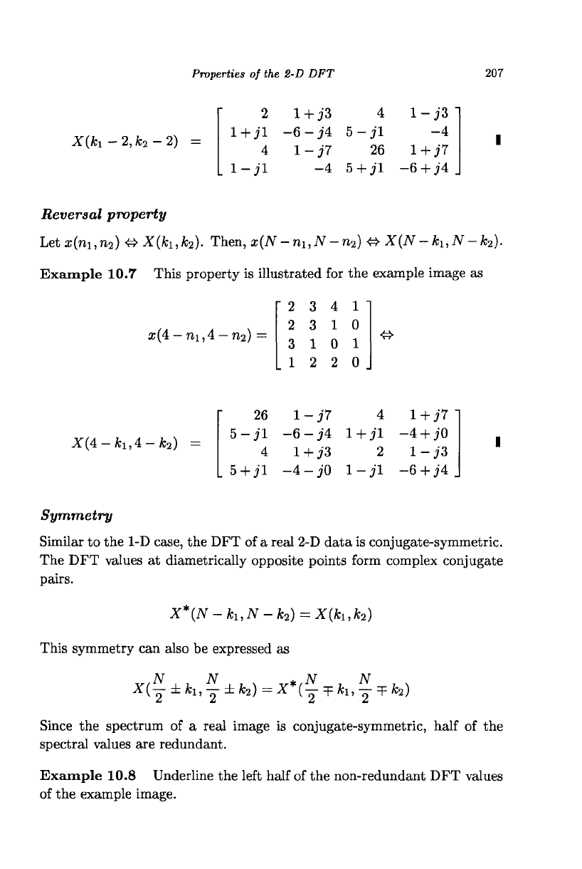
Properties of the 2-D DFT
207
X(fci-2,*
2
-2) =
2
+n
4
-jl
1 + J3
-6 - jl
1-J7
-4
4
5-jl
26
5 + jl
1-J3
-4
1+J7
-6+>4
Reversal property
Let ar(ni,n
2
)
<3>
X(fci, fc
2
). Then, ar(iV-n
u
N-n
2
)
<£>
X(N-k
u
N-k
2
).
Example 10.7 This property is illustrated for the example image as
•Y(4-fci,4-*2)
n
2
) -
26
5-jl
4
5 + jl
'234
2 3 1
3 1 0
.12 2
i-i7
-6 - j4
l+j'3
-4 - JO
1 "
0
1
0 .
>£>
4
l+jl
2
1-jl
1+J7
-4 + jO
1-J3
-6+j4
Symmetry
Similar to the 1-D case, the DFT of a real 2-D data is conjugate-symmetric.
The DFT values at diametrically opposite points form complex conjugate
pairs.
X*{N-k
1
,N-k
2
)
= X{k
u
k2)
This symmetry can also be expressed as
N N * N
X(-±k
1
,-±k
2
) = X*(-
T
k
1
,- + k
2
)
~2
Since the spectrum of a real image is conjugate-symmetric, half of the
spectral values are redundant.
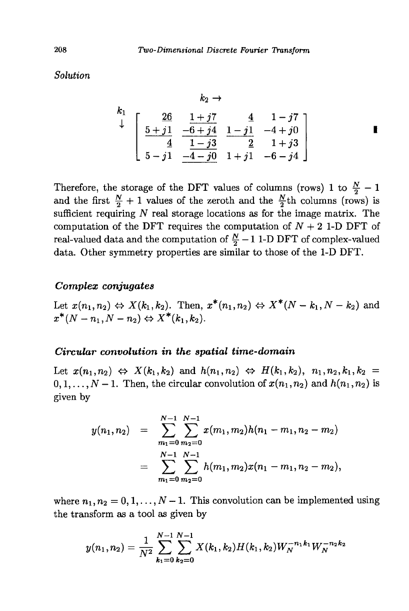
Example 10.8 Underline the left half of the non-redundant DFT values
of the example image.
208
Two-Dimensional Discrete Fourier Transform
Solution
*1
1
26
5+jl
4
L
5-jl
1 + J7
-6 + j4
1-J3
-4-jO
4
i-ii
2
1+jl
1-J7
-4 + jO
1+J3
-6-J4
Therefore, the storage of the DFT values of columns (rows) 1 to y - 1
and the first y + 1 values of the zeroth and the yth columns (rows) is
sufficient requiring TV real storage locations as for the image matrix. The
computation of the DFT requires the computation of N + 2 1-D DFT of
real-valued data and the computation of ^
—
1
1-D DFT of complex-valued
data. Other symmetry properties are similar to those of the 1-D DFT.
Complex conjugates
Let x(n
u
n
2
) •£> X(k
1
,k
2
). Then, x*(n
1
,n
2
)
<&
X*(N -ki,N - k
2
) and
x*(N-m,N- n
2
) O
X*(k
u
k
2
).
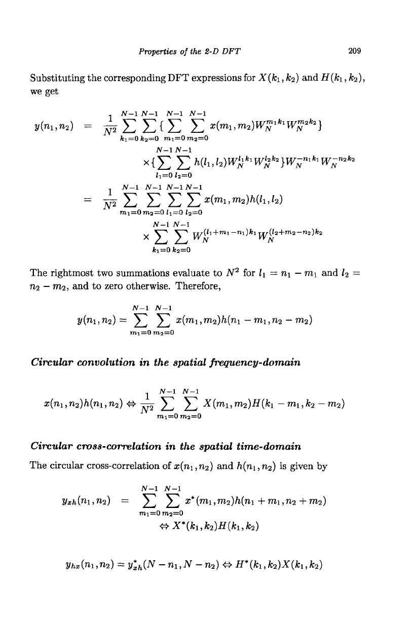
Circular convolution in the spatial time-domain
Let x(ni,n
2
) & X(ki,k
2
) and h(ni,n
2
) <S> H(ki,k
2
), ni,n
2
,ki,k
2
=
0,1,...,N
—
1. Then, the circular convolution of x(ni,n
2
) and h(ni,n
2
) is
given by
7V-1 N-l
y(ni,n
2
) = E ^2 x(mi,m
2
)h{ni-mi,n
2
-m
2
)
mi =0 7712=0
N-l N-l
= E E h(mi,m
2
)x(n\ —m\,n
2
—
m
2
),
7711=0 7712 = 0
where n\, n
2
=
0,1,...,
N - 1. This convolution can be implemented using
the transform as a tool as given by
1
N-I N-i
y{n
u
n
2
) = T^ E E X{k
u
k
2
)H{k
u
k
2
)W^W^
k
*
kl =0*2=0
Properties of the 2-D DFT 209
Substituting the corresponding DFT expressions for X(ki, k
2
) and H(ki, k
2
),
we get
y(n
u
n
2
) = ^ £ £^ £ E ^^W*
1
^*
2
}
fci=0fc
2
=0 mi=0roj=0
JV-l JV-l
x{j2 E M'i,/2)^
fci
t<
2
*
2
}^
nifci
w-"
2
*
2
l
1=
0h=0
-. JV-l JV-l N-1N-1
=
w E E E
E
af
(
mi
'
ma
W
i
'
Z2
)
mi=0 m
2
=0 (i=0 '2=0
jv-i Jv-i
V~* V~~*
TT^(ii
+ mi-ni)*iTi^((2+m2-n
2
)fc2
kl =0*2=0
The rightmost two summations evaluate to N
2
for li = ni
—
mi and
Z2
=
ri2
—
m
2
, and to zero otherwise. Therefore,
JV-l JV-l
y(ni,ri2) = £ E
x
i
m
i>
m
2:)h{ni—mi,n2
—
m2)
7711=0 7712=0
Circular convolution in the spatial frequency-domain
JV-l JV-l
x(ni,n
2
)h(ni,n
2
) <£> j= E ^2
x
{™
1
,m
2
)H{ki -
mi,k
2
- m
2
)
7711=0 7712=0
Circular cross-correlation in the spatial time-domain
The circular cross-correlation of x(ni,n
2
) and h(ni,n
2
) is given by
JV-l JV-l
Vxh{ni,n
2
) = £ y^ ar*(mi,m
2
)/i(ni+mi,n
2
+m
2
)
7711=0 7712=0
•»x*(*i,*
2
)ir(*i,fc2)
2/hx("i,n
2
) =
y*
xh
{N
- n
u
N -n
2
) & H*(k
1
,k
2
)X(k
l
,k
2
)
210
Two-Dimensional Discrete Fourier Transform
The autocorrelation operation is the same as the cross-correlation operation
with x{n\,ri2) = /i(ni,n
2
).
ifc*(ni,n
2
) = IDFT of
(\X(k
u
k
2
)\
2
)
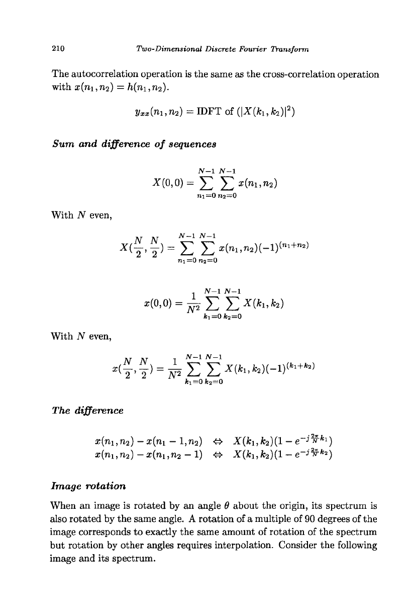
Sum and difference of sequences
N-l
JV-1
x(o,o)=
J2
E*-'
12
)
m=0 n2—0
With N even,
x
(f'Y)=EE^'^)(-
1
)
(
"
1+
"
2)
ni=0 ri2=0
1
JV-1 JV-1
fc, =0*2=0
With JV even,
fc
1=
0fc
2
=0
T/ie difference
x{ni,n
2
)-x{n
1
-l,n
2
) <3> X(fci,A;
2
)(l-e
-
^*
1
)
x(ni,n
2
)-x(n
1
,n
2
-1) <S> X(fci,fc
2
)(l -
e
-
^*
2
)
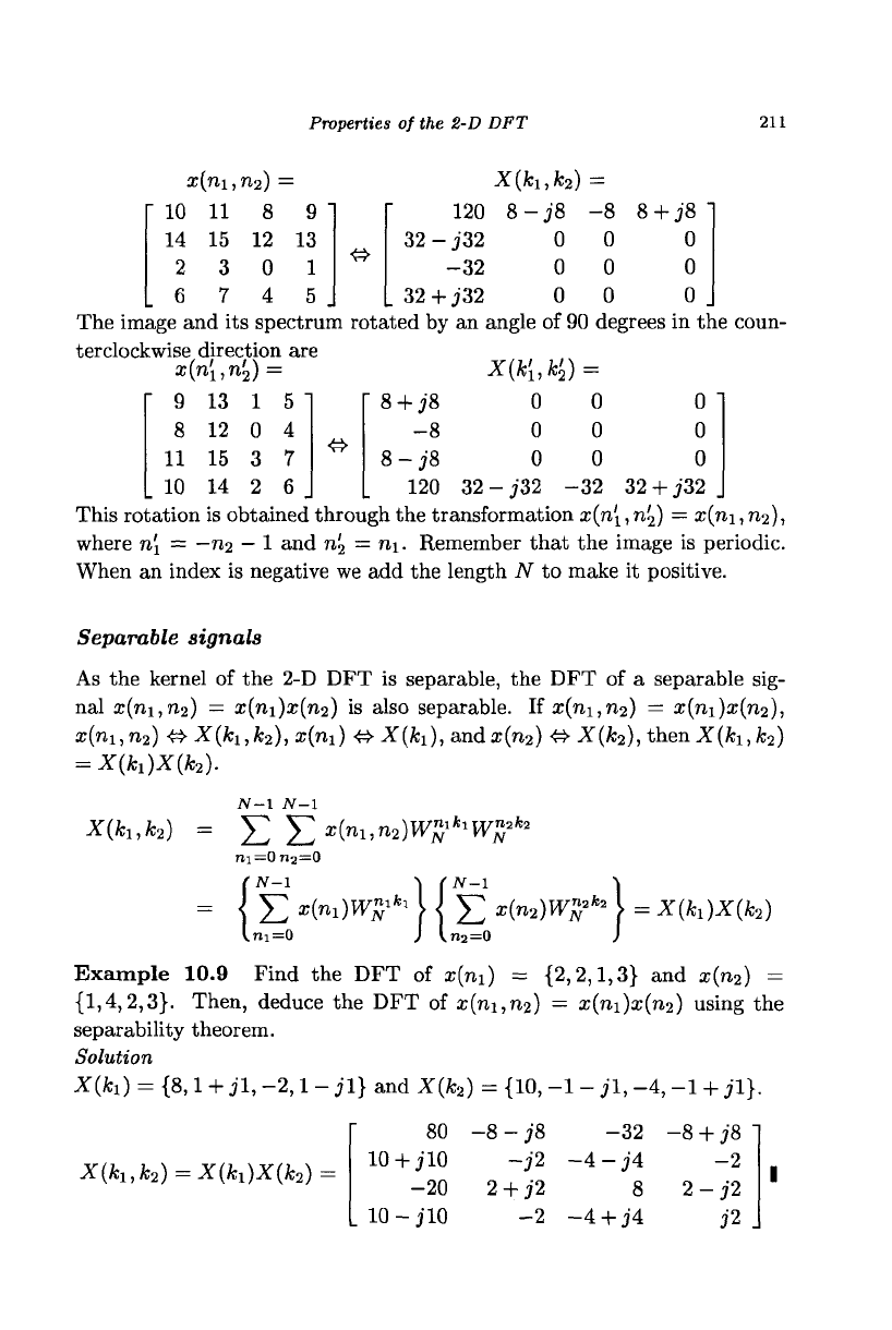
Image rotation
When an image is rotated by an angle 9 about the origin, its spectrum is
also rotated by the same angle. A rotation of a multiple of 90 degrees of the
image corresponds to exactly the same amount of rotation of the spectrum
but rotation by other angles requires interpolation. Consider the following
image and its spectrum.
Properties of the 2-D DFT
211
x(m,n
2
) =
10 11 8 9
14 15 12 13
2 3 0 1
6 7 4 5
<3>
9
8
11
10
13
12
15
14
1
0
3
2
5
4
7
6
&
8-j8
0
0
0
-8
0
0
0
8 + J8
0
0
0
angle of 90 degrees in t
X(ki, k
2
)
0
0
0
- J"32 -
=
0
0
0
32
0
0
0
32 + j32
X(k
u
k
2
) =
120
32 - j32
-32
L
32+J32
The image and its spectrum rotated by an
terclockwise direction are
x{n[,n'
2
) =
8 + j8
-8
8-J8
120 32
This rotation is obtained through the transformation
a^n'j,
n
2
) = x(ni, n
2
),
where n\ = —n
2
—
1 and n'
2
= ni. Remember that the image is periodic.
When an index is negative we add the length N to make it positive.
Separable signals
As the kernel of the 2-D DFT is separable, the DFT of a separable sig-
nal x(ni,n
2
) — x(ni)x(n
2
) is also separable. If x(rii,n
2
) = x(ni)x(n
2
),
x{ni,n
2
) & X(ki,k
2
), x{n,\)
<£>
X(ki), anda;(n2)
<=>
X(k
2
),
thenX(fci,fc
2
)
= X(k!)X{h2).
JV-1 N-l
X{k
u
k
2
) = J2 E <n
u
n
2
)W^W^
k
>
711=0 712=0
= ( Yl *(m W*
1
1
{
£
x(n
2
)Wtf
k
>
\
=
X(h)X(k,
l?ll=0 J (.712=0 J
Example 10.9 Find the DFT of x(m) = {2,2,1,3} and x(n
2
) =
{1,4,2,3}.
Then, deduce the DFT of x(ni,n
2
) = x(ni)x(n
2
) using the
separability theorem.
Solution
X(k
x
) = {8,1 + jl, -2,1 - jl} and X{k
2
) = {10, -1 - jl, -4, -1 + jl}.
X(k
1
,k
2
) = X(k
1
)X(k
2
)
80 -8-j8 -32 -8 + j8
10 + jlO -j2 -4-j4 -2
-20 2 + j2 8 2-J2
L 10-jlO -2 -4 + j4 j2 J
212
Two-Dimensional Discrete Fourier Transform
Parseval's theorem
This theorem implies that the sums of the squared magnitudes of the input
and DFT sequences are related by the constant factor TV
2
, the number of
samples. That
is
the signal power can also
be
computed from the DFT
coefficients of the input sequence.
N-l
N-l
1
JV-1
N-l
£
£
\x{n
u
n,)\*
=
± £ £
\X(
kl
,k
2
)f
ni=0n
2
=0 ki =0*2=0
Since the squared magnitude can
be
computed
by
multiplying
a
complex
number by its conjugate, we can write the left summation
as
JV-l
N-l
^
^
a;(ni,n
2
)x*(ni,n
2
)
r»i=0n2=0
Substituting
the
corresponding IDFT expressions
for
2(7x1,712)
and
x*
(711,712),
and rearranging the summations, we get
1
N-l N-l N-l N-l N-l N-l
W£
£ £
£*(*!, W(*3,fc
4
)
£
^W-^r-^W-n^-k.)
fc
1=
0 *
2
=0 fc
3
=0 fc
4
=0 ni=On
2
=0
If
fci
=
£3 and A2
= ki,
this expression becomes
fc
1=
0fe
2
=0 fci=0fe
2
=0
Otherwise, the expression evaluates
to
zero. The generalized form
of
this
theorem applies for two different signals as given by
JV-l
N-l
1
N-l N-l
E
E
a;
(
n
i'
n
2)2/*(ni,n
2
) = jyj
E E
X
(
fcl
'
fc2
)
y
*(
fcl
'
fc2
)
ni=0n
2
=0 *M=0fc
2
=0
10.5 The 2-D PM DFT Algorithms
The DFT
of
2-D data
is
usually obtained
by
computing the 1-D DFT
of
each row of data followed by the 1-D DFT
of
each column of the resulting
data and vice versa. The SFG
of a
2-D DFT algorithm with
the
same
The 2-D PM DFT Algorithms
213
R_vector R_stage 1 R_stage 2 Rjstage 3 Col_by_Col
o(0) =
a;(0,0) ± x(0,8)
o(4) =
x(0,4) ± x(0,12)
a(2) =
ar(0,2) ± ar(0,10)
o(6)=o
x(0,6)±x(0,14)
o(l) =
x(0,l)±x(0,9)
o(5) =
x(0,5) ± x(0,13)
o(3) =
x(0,3) ± x(0,ll)
o(7)=o
x(0,7) ± x(0,15)
f
A(0) =
,
OX(0,0),I(0,8)
, Mi) =
1X(0,1),X(0,9)
,
A{
?) =
2X(0,2),X(0,10)
t
A(3) =
'3X(0,3),X(0,11)
A(4) =
X(0,4),X(0,12)
A(5) =
X(0,5),X(0,13)
A(6) =
X(0,6),X(0,14)
A{7) =
X(0,7),X(0,15)
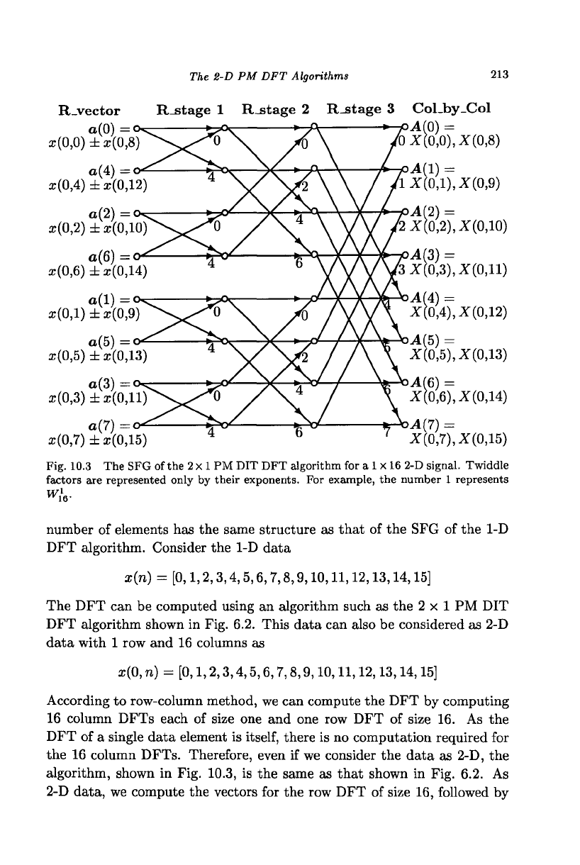
Fig. 10.3 The SFG of the
2
x
1
PM DIT DFT algorithm for a
1 X
16 2-D signal. Twiddle
factors are represented only by their exponents. For example, the number 1 represents
number of elements has the same structure as that of the SFG of the 1-D
DFT algorithm. Consider the 1-D data
x{n) = [0,1,2,3,4,5,6,7,8,9,10,11,12,13,14,15]
The DFT can be computed using an algorithm such as the 2x1 PM DIT
DFT algorithm shown in Fig. 6.2. This data can also be considered as 2-D
data with 1 row and 16 columns as
x(0,
n) = [0,1,2,3,4,5,6,7,8,9,10,11,12,13,14,15]
According to row-column method, we can compute the DFT by computing
16 column DFTs each of size one and one row DFT of size 16. As the
DFT of a single data element is
itself,
there is no computation required for
the 16 column DFTs. Therefore, even if we consider the data as 2-D, the
algorithm, shown in Fig. 10.3, is the same as that shown in Fig. 6.2. As
2-D data, we compute the vectors for the row DFT of size 16, followed by