Szilas A.P. Production and transport of oil and gas, Gathering and Transportation
Подождите немного. Документ загружается.

230
7
PIPELINE
TRANSPORTATION
OF
OIL
The inside and outside wall temperatures of steel pipe are taken to be equal, that is,
7;=
r,.
The multiple equation
7.6- 3
1
may be decomposed into three independent
equations:
k(
T,
-
7;)
=
a
I
din(
7''
-
7;)
7.6
-
32
27&(
r,
-
7J
din
a,d,n(T'-
7;)=
~
~~___
1
n,
7.6
-
33
4
sr,d,n(T,-
TJ=a,dinrc(Tn-
T,).
7.6
-
34
The relationship needed to determine
7;
is
Eq.
7.6
-
32.
The calculation can be
performed by successive approximations.
A
value for is assumed first, and, using
it,
the physical parameters
of
the
oil
required to calculate
N,,N,,
and
NNu
,
are
established.
As
a result. Eq.
7.6-
18
will furnish a value for
a,
.
Introducing this into
Eq.
7.6
-
17,
a k-value is calculated. Now Eq.
7.6
-
32
is used to produce another
k-
value, likewise using the previously determined
a,
.
If
the
ks
furnished by the two
procedures agree, then the value assumed for
7;
is correct.
If
this is not the case,
calculation has to
be
repeated with a different value for
r.
-
Equation
7.6
-
33
or
k'
W/
m'
K
2
1
12
3
1,
5
6
78
0
lOlll?
Month
1066
1867
raw
0
8
A
pipllw
b
A
AS
;
:
0
.C
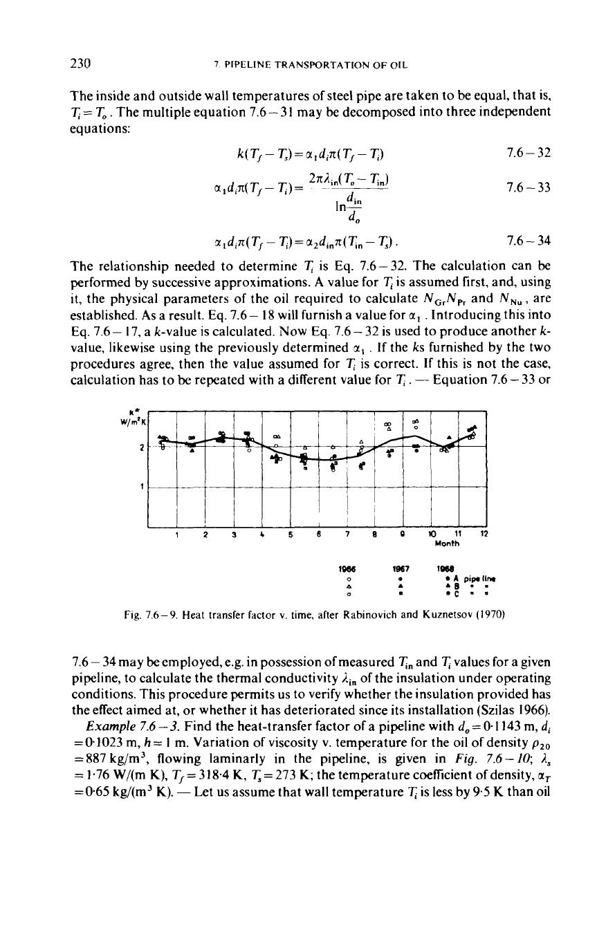
Fig.
7.6-9.
Heat transfer
Factor
v.
time. after Rabinovich and Kuznetsov
(1970)
7.6
-
34
may be employed, e.g. in possession of measured
Tn
and
7;
values for a given
pipeline, to calculate the thermal conductivity of the insulation under operating
conditions. This procedure permits us to verify whether the insulation provided has
the effect aimed at, or whether
it
has deteriorated since its installation (Szilas
1966).
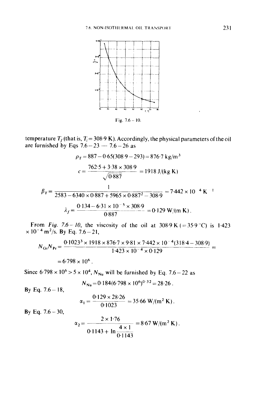
Example
7.6-3.
Find the heat-transfer factor of a pipeline with
d,=0-1143
m,
di
=01023
m,
h
=
1
m. Variation of viscosity v. temperature for the oil
of
density
pzo
=887
kg/m3, flowing laminarly in the pipeline, is given in
Fig.
7.6-10;
A,
=
1.76
W/(m
K),
T,=318.4
K,
T,=273
K;
the temperature coefficient
of
density,
aT
=065
kg/(m3
K).
-
Let us assume that wall temperature is less by
9.5
K
than oil
7
6.
NON-ISOTtICRMAI.
011.
TKAIUSI'OKI
23
1
Fig.
7.6
-
10.
temperature T,(that is,
7;=
308.9
K).
Accordingly, the physical parameters
of
the
oil
are furnished by
Eqs
7.6
-
23
-
7.6
-
26
as
pT=
887-0.65(308.9-293)=876.7
kg/rn-'
762.5
+
3.38
x
308.9
C=
=
1918
J/(kg
K)
Jo887
1
=7.442~
10
K
'
IOT
=
2583
-
6340 x 0.887
+
5965
x
0887'
-
308.9
0.134-6.31
x
10
x
308.9
0.887
=O.I29
W,/(rn
K)
).,
=
______~~
~~~
-~
From
Fig.
7.6-
10,
the viscosity
of
the
oil
at
308.9
K
(=
35.9
"C)
is
1.423
0.1
0233
x
19 18
x
876.7
x
9.8
1
x
7.442
x
10
4(
3 18.4
-
308.9)
1.423
x
lo-"
x
0.129
x
m2/s.
By
Eq.
7.6-21,
- -
NGrNpr=
~~
=
6.798
x
1
O6
.
Since
6.798
x
lo6>
5
x
lo4,
NN,
will
be
furnished
by
Eq.
7.6-22
as
NN,
=0.184(6.798
x
10')'
32
=
28.26.
By
Eq.
7.6- 18,
0.129
x
28.26
0.1023
a,
=
=
35.66
W/(m2
K)
By
Eq.
7.6
-
30,
2
x
1.76
4x1
0.1
143
+
In
~
0.1 143
a,=
~
=
8.67
W/(m2
K)
.
232
7.
PIPELINE TRANSPORTATION
OF
011.
Now the heat-transfer factor is, by
Eq.
7.6- 17,
7L
k=
=
2.448 W/(m
K)
1
1
+-
35.66
x
0.
I023
8.67
x
0.
I
143
whereas
Eq.
7.6
-
32 yields
0.1023
x
7~
x
35'66(318.4-308.9)
318
x
4-273
k=
=
2.400 W/(m
K)
.
As
a further approximation, let 7;=308.7
K,
in which case
Eq.
7.6-- 17 yields
2.449
W/(m
K),
and
Eq.
7.6
-
32 yields 2.450,
so
that
k
=
2.45 W/(m
K)
is accepted.
7.6.4.
Calculating the head
loss
for
the steady-state
flow
(a)
The oil is Newtonian
(A)
Chernikin's theory
Equation 7.6-2 will hold
for
an infinitesimal length dl
of
pipeline only, as the
temperature
of
the
oil
flowing through the pipe may
be
considered constant, and
so
may, in consequence, also
,I
and
v:
E.llZ
dh
-
--
dl.
*
-
2gd,
Equation
1.1
-
10
may be used
to
express
1.
also for laminar flow:
7.6
-
35
7.6
-
36
where
a
and
b
are constants that, in laminar flow, depend on the flow type only.
Substituting this expression
of
2
and the expression
7.6
-
37
where the constant coeflicient is
7 h
NON-ISOTHERMAL
OIL
TRANSPORT
233
Viscosity
v.
temperature
in
a Newtonian oil may be described over a limited
temperature range also by Filonov's explicit formula
,!
=
y"p
-
n"
7.6
-
38
where
vo
is kinematic viscosity at
0
'
C
and
where
11,
and
vI,
are experimeritally determined viscosities at the temperatures
7;
and
7;,
.
Let us point out that Tis to be written
in
"C.
vo
may be considered as a fictive,
extrapolated value.
It
has no physical meaning unless the oil is Newtonian al the
temperature considered.
At
a distance
1
from the head end of the pipeline. the
temperature
of
the flowing oil is expressed by Eq.
7.6
-
I5
as
where
k
4PC
Introducing this into Eq.
7.6-38,
we obtain
m=-,
Substituting this latter equation
in
Eq.
7.6-37,
we get
7.6
-
39
Let
hn(
T,
,
~
7J
=
B,
and
then
I
h
-
S
ACR'
'"'dl.
r-
0
Let Be-"'=u; then, e-"'=u/B. Hence,
1u
I
mB
mu
I=
-
-In-
and dl=
-
-du
Substituting the constants into this equation yields
R
234
7.
PIPELINE TRANSPORTATION
OF
OIL
Since
a,
we have, in the original notation,
x
.(
Ei
[
-
hn(
T,
-
T,)]
-
Ei
[
-
hn(
T,
-
'Qe-
'"'1
).
.
Introducing the
vo=v,
enTJl
implied by Eq. 7.6-38, and the
(T,
-
T,)e-'"'=
T,,
-
T,
implied by Eq. 7.6-
15,
we arrive at
q(2-b)vb ebn(TJI
-
T.)
X
hl=P-p+
ml
x
(Ei[
-
hn(7''
-
T,)]
-
Eill-hn(Tl,
-
T,)I)
.
This equation may be contracted to read
7.6
-
40
7.6-41
in which case, with reference to Eq. 7.6- 37,
it
may be interpreted as the product of
the pressure head
loss
of a liquid in isothermal flow whose viscosity is
v1
at the head
end of the pipeline, of the correction accounting for cooling along the pipeline
section
A,
and of the radial temperature correction
A,.
In
laminar flow,
=
128/ng,
and
b=
I;
in turbulent flow, the corresponding values are 0.20l/y and
0.25,
if
friction factor
I
is determined using Eq.
1.1
-4 (Chernikin
1958).
In Eq. 7.6
-41,
ebn(Tfr
-
T.4
A,
=
(Ei[
-
bn(T,
-
T,)]
-
Ei[
-
hn(T12
-
T,)]}
ml
A,
is, then, the correction factor accounting for axial cooling.
It
shows how many
times the head
loss
is increased owing to the fact that oil temperature gradually
decreases from
T,
to
TJ2
during flow.
A,
is the correction factor accounting for
radial cooling. Its value would
be
unity
if
oil temperature were constant over any
pipeline cross section. However, temperature in effect decreases from the pipe axis
towards the wall (cf. e.g. Example 7.6-4), and hence mean viscosity
in
the pipe is
higher than the axial viscosity.
A,
accounts for this effect. Chernikin makes use of the
Sieder-Tate relationship
0
A,
=
E
(;)
7.6
-
42
7.6.
NON-ISOTHERMAL OIL TRANSPORT
235
viand
vf
are average viscosities of oil at the pipe wall and along the axis, respectively,
at the arithmetic average
of
the head-end and tail-end temperatures of the pipeline
section considered;
E
and
w
are constants
(E
is
0.9
in laminar and
1
in turbulent flow;
o
ranges from
1/3
to
1/4
in laminar and from
1/3
to
1/7
in turbulent flow). In
pipelines transporting viscous crudes, the transition from laminar to turbulent flow
may be expected at about
N,,
=
2000.
Equation
7.6
-
41,
suitable for comparatively fast calculation, has the following
limitations.
(i)
In calculating the friction factor of turbulent flow,
it
employs the
Blasius equation which refers to smooth pipe. Accuracy is easy to improve by
introducing different constants
a
and
b
(cf. e.g. Eq.
7.4.
-
8).
(ii)
Equation
7.6
-
38
is
an approximate expression of the temperature-dependence of oil viscosity, valid
over a rather limited temperature range only.
(iii)
Constants
E
and
w
have rather
broad ranges and therefore
A,
cannot be determined to a desirable degree of
accuracy.
(B)
Ford's
theory
(with
modification)
This procedure, more lengthy than the foregoing one, establishes the head
loss
of
oil flowing
in
a
pipeline by a finite-difference procedure. It permits
us
to account for
the variation in
k,
and to use accurate friction-factor and viscosity values (Ford
1955).
Below we shall present this method in a slightly modified form.
Starting from the initial axial oil temperature
Tf,,
we assume an axial
temperature drop
ATf
of a few
"C
to take over a place comparatively short, as yet
unspecified length
I,
of pipe. It is assumed that the average temperature over this
length of pipe is, in a fair approximation,
Tj
1
=
Tf
I
-0'5ATf.
7.6
-
43
Using Eqs
7.6-
15,
7.6- 17
and
7.6- 30,
it is possible to calculate the length
I,
over
which the axial temperature drop is precisely
ATf.
In order to perform the
calculation it is necessary to determine the heat transfer factor as indicated in
Example
7.6
-
3
and, in the process, to find also the average wall temperature
'&.,
.
Continuing the process, one obtains related values of
Tf
,7;,
Tn
and
I,
which permits
plotting graphs of temperature v. length.
Viscosity values corresponding to the Reynolds number
N,,
=
2000,
characteriz-
ing the transition from laminar to turbulent flow, are calculated using Eq.
1.1
-
2;
oil
temperature
Tf
corresponding to the 'critical' viscosity of the oil to be conveyed is
then read
off
the corresponding
T-v
graph. The point along the line where this
temperature sets in will be where turbulent flow passes into laminar. In turbulent
flow, as far as head
loss
calculations are concerned, pipeline cross-section
temperature may be equated with
Tf
.
In laminar flow, however, the temperature
differential between pipe axis and pipe wall is
so
significant that the average of the
two, which will in fact determine the behaviour
of
the crude (its effective viscosity
first of all), has to be determined separately.
It
was found in practice that this is done
most simply by reading said temperature
off
the experimentally established diagram
236
7
PIPE1
1NF TRANSPORTATION
OF
OII
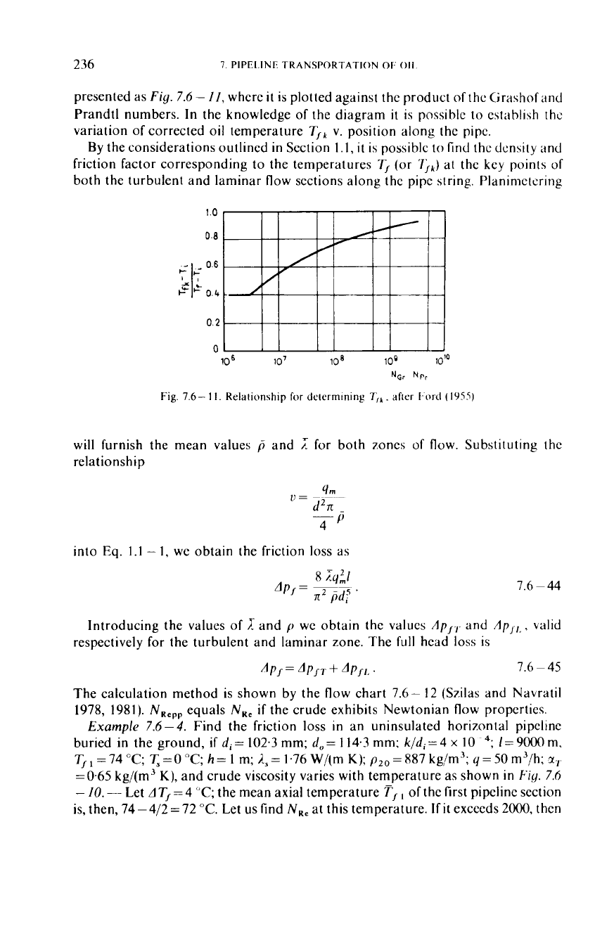
presented as
Fig.
7.6
-
II,
where
it
is plotted against the product of thc Grashof and
Prandtl numbers. In the knowledge of the diagram
it
is possible to establish
the
variation
of
corrected oil temperature Tfk
v.
position along the pipc.
By
the considerations outlined
in
Section
1.1,
it
is
possiblc
to find thc dcnsity and
friction factor corresponding to the temperatures
T,
(or
7jk)
at the key points of
both the turbulent and laminar flow sections along the pipe string. Planinietering
NGr
Nf'r
Fig.
7.6-
1
I.
Relationship
for
determining
7,,
.
after
I.ord
(1955)
will
furnish the mean values
p
and
relationship
for both zones of flow. Substituting
thc
into
Eq.
1.1
-
I,
we obtain the friction
loss
as
1.6
~ 44
Introducing the values of
and
p
we obtain the values
Ap,.,.
and
A~j1,
,
valid
respectively for the turbulent and laminar zone. The
full
head
loss
is
4/=
&,I
+
AP,,
'
1.6
~
45
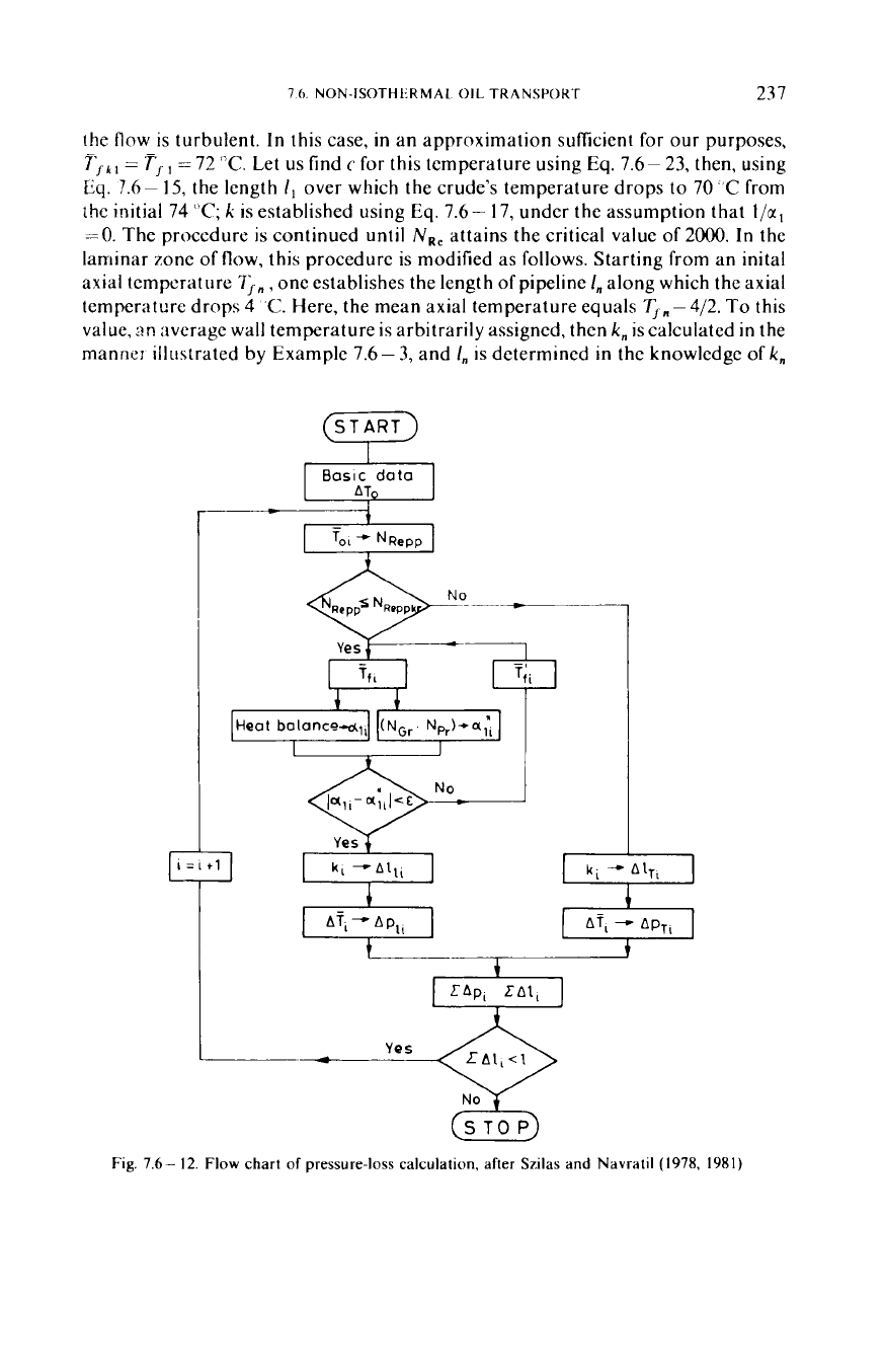
The calculation method is shown by the flow chart
7.6
-
12
(Szilas and Navratil
1978, 1981).
NRepp
equals
NR,
if
the crude exhibits Newtonian flow properties.
Example
7.6-4.
Find the friction
loss
in
an uninsulated horizontal pipeline
buried in the ground,
if
di
=
102.3
mm;
do
=
1
14.3
mm;
k/dj=
4
x
10
~
4;
I=
9000
m,
TJ,=74"C;
T,=O"C;h=l
m;i,,=1~76W/(mK);p,,=887kg/m';;=50m3/h;r,
=0.65
kg/(m3
K),
and crude viscosity varies
with
temperature as shown
in
Fig.
7.6
-
10.
-
Let
AT,=4
"C;
the mean axial temperature
TJ,
of the first pipeline section
is, then,
74-4/2=72 "C.
Let
us
find
NR,
at this temperature.
Ifit
exceeds
2000,
then
7
h
NON-ISOTH1:RMAL
OIL
TRANSPORT
237
Heat
bolance-d,,
the
flow
is turbulent. In this case, in an approximation suflicient
for
our
purposes,
7';
kl
=
Tf
I
=
72
"C.
Let
us
find
c
for this temperature using Eq. 7.6- 23, then, using
Eq.
!.6-
15,
the length
I,
over which the crude's temperature drops to 70°C from
the initial 74
"C;
k
is established using Eq. 7.6- 17, under the assumption that
I/@,
=O.
The procedure is continued until
N,,
attains the critical value of 2000.
In
the
laminar zone of
flow,
this procedure is modified as follows. Starting from an inital
axial temperature
7;,,
,
one establishes the length of pipeline
I,,
along which the axial
temperaturc
drops
4
'C.
Here, the mean axial temperature equals
Tf,-4/2.
To
this
value,
an
average wall temperature is arbitrarily assigned, then
k,
is calculated
in
the
mannz: illustrated by Example 7.6
-
3, and
I,
is determined in the knowledge
of
k,
(NGr
Np,)+a:,
Basic
data
238
a
0
10
0
08
0
06
0
04
002
0
01
-
-
-
-
-
-
-
3 13.6
309.6
305.6
301.6
297.7
294.1
Fig. 7.6
-
I3
345.0
34
1
.O
337.0
333.0
329.0
325.0
321.7
308.7
305.1
301.6
298.1
294.6
291.3
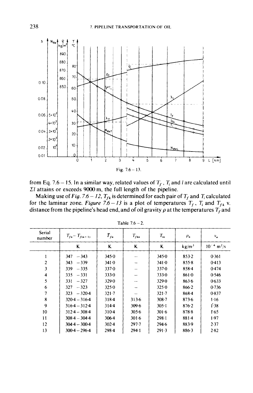
from
Eq.
7.6
-
15.
In a similar way, related values of
7”
,
7;
and
I
are calculated
until
CI
attains
or
exceeds
9000
m, the
full
length of the pipeline.
Making use
of
Fig.
7.6
-
12,
T,,
is determined
for
each pair of
T,
and
7;
calculated
for
the laminar zone.
Figure
7.6
-
I3
is a plot of temperatures
T,
,
and
T,,
v.
distance from the pipeline’s head end, and of oil gravity pat the temperatures
T,
and
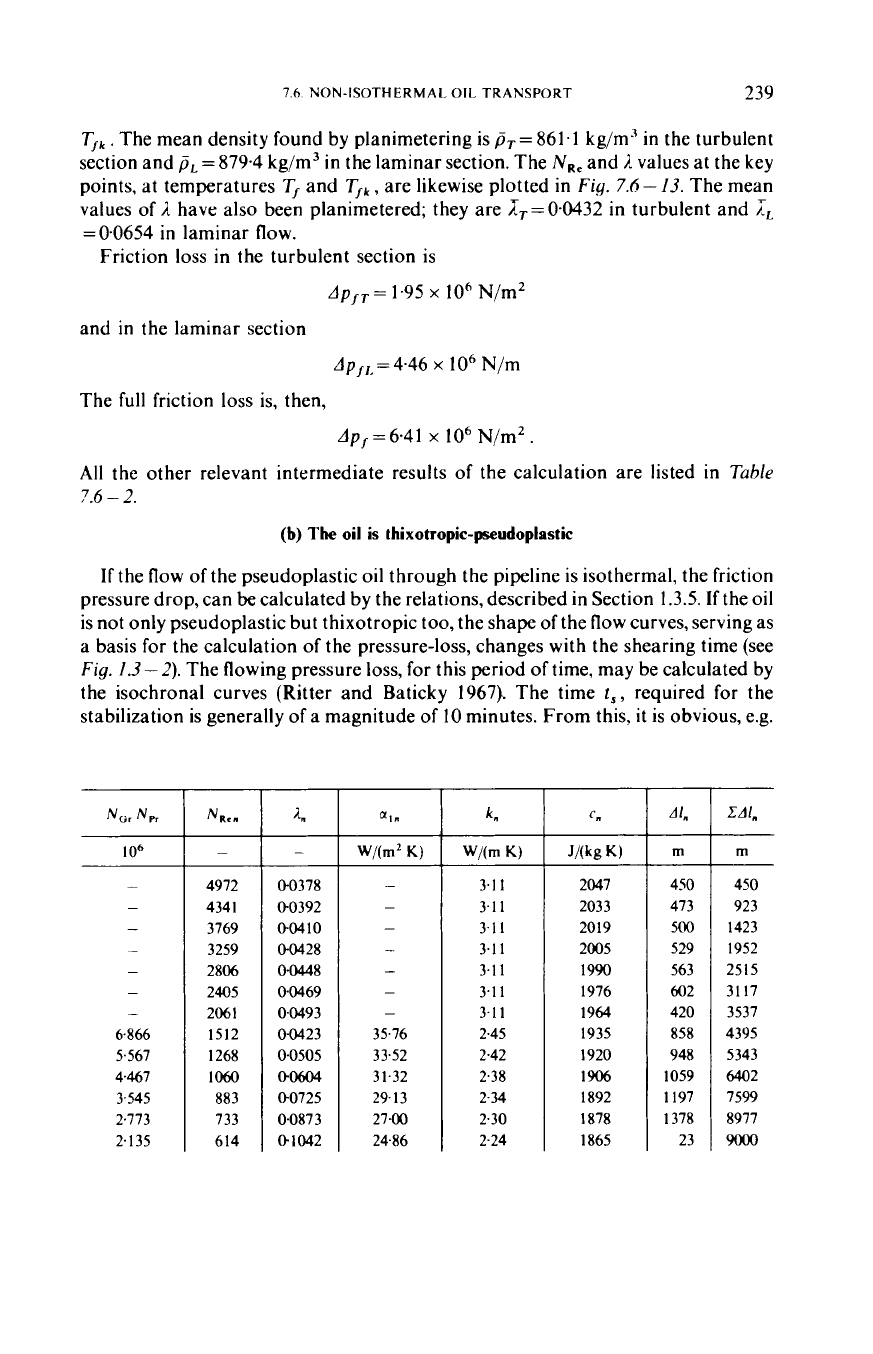
Table 7.6
-
2.
Serial
number
1
2
3
4
5
6
7
8
9
10
11
12
13
K
347 -343
343 -339
339 -335
335 -331
331 -327
327 -323
323 -320.4
320.4
-
3
16.4
3 16.4
-
3 12.4
3 12.4
-
308.4
308.4
-
304.4
304.4
-
300.4
300.4
-
296.4
T/”
K
345-0
34
1
.O
337.0
333.0
329.0
325.0
321.7
3 18.4
3 14.4
3 10.4
306.4
302.4
298.4
P.
853.2
858.4
855.8
86
I
.O
863.6
866.2
868.4
873.6
876.2
878.8
883.9
886.3
881.4
m‘js
0361
0.413
0474
0.546
0.633
0.736
0,837
1.16
1-38
r.65
I
.97
2.37
2.82
7.6
NON-ISOTHERMAL OIL TRANSPORT
239
A/,
rn
450
473
500
529
563
602
420
858
948
1059
1197
1378
23
T,,
.
The mean density found by planimetering is
PT=
861.1
kg/m3
in
the turbulent
section and
pL
=
879.4
kg/m3 in the laminar section. The
N,,
and 1. values at the key
points, at temperatures
T,
and
T,,
,
are likewise plotted in
Fig.
7.6
-
13.
The mean
values of
,I
have also been planimetered; they are
IT
=
0.0432 in turbulent and
LL
=0.0654
in
laminar flow.
Friction
loss
in the turbulent section is
Ap,,=
1.95
x
10'
N/m2
and
in
the laminar section
Ap,,,
=
4.46
x
lo6
N/m
The full friction
loss
is, then,
ZAl,
m
450
923
1423
1952
2515
3117
3537
4395
5343
6402
7599
8977
9ooo
dp,=6.41
x
lo6
N/m2.
-
I
O6
All
the other relevant intermediate results of the calculation are listed
in
Table
7.6
-
2.
-
(b)
The oil
is
thixotropic-pseudoplastic
If
the flow
of
the pseudoplastic oil through the pipeline is isothermal, the friction
pressure drop, can
be
calculated by the relations, described in Section
1.3.5.
If
the oil
is not only pseudoplastic but thixotropic too, the shape
of
the flow curves, serving as
a basis
for
the calculation
of
the pressure-loss, changes with the shearing time (see
Fig.
1.3-2).
The flowing pressure loss, for this period
of
time, may be calculated by
the isochronal curves (Ritter and Baticky
1967).
The time
t,,
required for the
stabilization is generally
of
a magnitude
of
10
minutes. From this.
it
is obvious, e.g.
4972
4341
3769
3259
2806
2405
2061
1512
1268
1060
883
733
614
00378
00392
00410
04428
04W8
0.0469
00493
0-0423
0.0505
00604
00725
0.0873
01042
-
-
-
-
-
-
-
6.866
5.567
4.467
3.545
2.773
2135
-
-
-
-
-
-
-
35.76
33.52
31.32
29.13
27.00
24.86
3.1
1
3.1
1
3.1
I
3.1
1
3.1
1
3.1
1
3.1
1
2.45
2.42
2.38
2.34
2.30
2.24
JAkg
K)
2047
2033
2019
2005
1990
1976
1964
1935
1920
1906
I892
1878
1865