Trauth M.H., MATLAB® Recipes for Earth Sciences, Third edition
Подождите немного. Документ загружается.

68 3 UNIVARIATE STATISTICS
corg1 and corg2 at an alpha=0.05 or a 5 % signi cance level. MATLAB
also provides a one-sample variance test
vartest(x,variance) analo-
gous to the one-sample t-test discussed in the previous section. e one-
sample variance test, however, virtually performs a χ
2
-test of the hypothesis
that the data in the vector
x come from a normal distribution with a vari-
ance de ned by
variance. e χ
2
-test is introduced in the next section.
e command
[h,p,ci,stats] = vartest2(corg1,corg2,0.05)
yields
h =
0
p =
0.7787
ci =
0.6429 1.8018
stats =
fstat: 1.0762
df1: 59
df2: 59
e result h=0 means that we cannot reject the null hypothesis without an-
other cause at a 5 % signi cance level. e p-value of 0.7787 means that the
chances of observing more extreme values of F than the value in this exam-
ple, from similar experiments, would be 7,787 in 10,000. A 95 % con dence
interval is [–0.6429 1.8018], which includes the theoretical (and hypoth-
esized) ratio
var(corg1)/var(corg2) of 1.2550
2
/1.2097
2
=1.0762.
We now apply this test to two distributions with very di erent standard
deviations, 1.8799 and 1.2939.
clear
load('organicmatter_five.mat');
We again compare the calculated Fcalc with the critical Fcrit at a 5 %
signi cance level, using the function
finv to compute Fcrit.
s1 = std(corg1);
s2 = std(corg2);
df1 = length(corg1) - 1;
df2 = length(corg2) - 1;

3.7 THE F-TEST 69
3 UNIVARIATE STATISTICS
if s1 > s2
slarger = s1;
ssmaller = s2;
else
slarger = s2;
ssmaller = s1;
end
Fcalc = slarger^2 / ssmaller^2
Fcrit = finv(1-0.05/2,df1,df2)
and get
Fcalc =
3.4967
Fcrit =
1.6741
Since the Fcalc calculated from the data is now larger than the critical
Fcrit, we can reject the null hypothesis. e variances are therefore di er-
ent at a 5 % signi cance level.
Alternatively, we can apply the function
vartest2(x,y,alpha),
performing a two-sample F-test on the two independent samples
corg1
and
corg2 at an alpha=0.05 or a 5 % signi cance level.
[h,p,ci,stats] = vartest2(corg1,corg2,0.05)
yields
h =
1
p =
3.4153e-06
ci =
2.0887 5.8539
stats =
fstat: 3.4967
df1: 59
df2: 59
e result h=1 suggests that we can reject the null hypothesis. e p-value
is extremely low and very close to zero suggesting that the null hypoth-
esis is very unlikely. e 95 % con dence interval is [2.0887 5.8539], which
again includes the theoretical (and hypothesized) ratio
var(corg1)/
var(corg2)
of 1.8799
2
/1.2939
2
=1.0762.

70 3 UNIVARIATE STATISTICS
3.8 The χ
2
-Test
e χ
2
-test introduced by Karl Pearson (1900) involves the comparison of
distributions, allowing two distributions to be tested for derivation from
the same population. is test is independent of the distribution that is be-
ing used, and can therefore be used to test the hypothesis that the observa-
tions were drawn from a speci c theoretical distribution.
Let us assume that we have a data set that consists of multiple chemical
measurements from a sedimentary unit. We could use the χ
2
-test to test the
null hypothesis that these measurements can be described by a Gaussian
distribution with a typical central value and a random dispersion around
it. e n data are grouped in K classes, where n should be above 30. e
frequencies within the classes O
k
should not be lower than four, and should
certainly never be zero. e appropriate test statistic is then
where E
k
are the frequencies expected from the theoretical distribution
(Fig. 3.12). e null hypothesis can be rejected if the measured χ
2
is higher
than the critical χ
2
, which depends on the number of degrees of freedom
Φ=K–Z, where K is the number of classes and Z is the number of param-
eters describing the theoretical distribution plus the number of variables
(for instance, Z=2+1 for the mean and the variance from a Gaussian distri-
bution of a data set for a single variable, Z=1+1 for a Poisson distribution
for a single variable).
As an example, we can test the hypothesis that our organic carbon mea-
surements contained in organicmatter_one.txt follow a Gaussian distribu-
tion. We must rst load the data into the workspace and compute the fre-
quency distribution
n_obs for the data measurements.
clear
corg = load('organicmatter_one.txt');
v = 9.40 : 0.74 : 14.58;
n_obs = hist(corg,v);
We then use the function normpdf to create the expected frequency distri-
bution
n_exp with the mean and standard deviation of the data in corg.
n_exp = normpdf(v,mean(corg),std(corg));
3 UNIVARIATE STATISTICS
3.8 THE
χ
2
-TEST 71
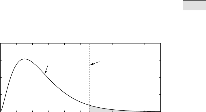
Reject the null hypothesis!
This decision has a 5%
probability of being wrong.
Don’t reject the
null hypothesis
without another cause!
02468101214161820
0
0.05
0.1
0.15
0.2
f( )
χ
2
χ
2
Φ =5
χ
2
(Φ=5, α=0.05)
Probability Density Function
Fig. 3.12 Principles of a χ
2
-test. e alternative hypothesis that the two distributions are
di erent can be rejected if the measured χ
2
is lower than the critical χ
2
. χ
2
depends on
Φ=K–Z, where K is the number of classes and Z is the number of parameters describing the
theoretical distribution plus the number of variables. In the example, the critical χ
2
(Φ=5,
α=0.05) is 11.0705. Since the measured χ
2
=6.0383 is below the critical χ
2
, we cannot reject
the null hypothesis. In our example, we can conclude that the sample distribution is not
signi cantly di erent from a Gaussian distribution.
e data need to be scaled so that they are similar to the original data set.
n_exp = n_exp / sum(n_exp);
n_exp = sum(n_obs) * n_exp;
e rst command normalizes the observed frequencies n_obs to a total
of one. e second command scales the expected frequencies
n_exp to the
sum of
n_obs. We can now display both histograms for comparison.
subplot(1,2,1), bar(v,n_obs,'r')
subplot(1,2,2), bar(v,n_exp,'b')
Visual inspection of these plots reveals that they are similar. It is, howev-
er, advisable to use a more quantitative approach. e χ
2
-test explores the
squared di erences between the observed and expected frequencies. e
quantity
chi2calc is the sum of the squared di erences divided by the
expected frequencies.
chi2calc = sum((n_obs - n_exp).^2 ./ n_exp)
chi2calc =
6.0383
72 3 UNIVARIATE STATISTICS
e critical chi2crit can be calculated using chi2inv. e χ
2
-test re-
quires the number of degrees of freedom Φ. In our example, we test the hy-
pothesis that the data have a Gaussian distribution, i. e., we estimate the two
parameters μ and σ. e number of degrees of freedom is Φ=8–(2+1)=5.
We can now test our hypothesis at a 5 % signi cance level. e function
chi2inv computes the inverse of the χ
2
CDF with parameters speci ed by
Φ for the corresponding probabilities in p.
chi2crit = chi2inv(1-0.05,5)
chi2crit =
11.0705
Since the critical chi2crit of 11.0705 is well above the measured chi2calc
of 5.4256, we cannot reject the null hypothesis without another cause. We can
therefore conclude that our data follow a Gaussian distribution. Alternatively,
we can apply the function
chi2gof(x) to the sample. e command
[h,p,stats] = chi2gof(corg)
yields
h =
0
p =
0.6244
stats =
chi2stat: 2.6136
df: 4
edges: [9.417 10.960 11.475 11.990 12.504 13.018 13.533 14.5615]
O: [8 8 5 10 10 9 10]
E: [7.0506 6.6141 9.1449 10.4399 9.8406 7.6587 9.2511]
e function automatically de nes seven classes instead of the eight classes
that we used in our experiment. e result
h=0 means that we cannot reject
the null hypothesis without another cause at a 5 % signi cance level. e p-
value of 0.6244 means that the chances of observing either the same result
or a more extreme result, from similar experiments in which the null hy-
pothesis is true, would be 6,244 in 10,000. e structure array
stats con-
tains the calculated χ
2
, which is 2.6136 and di ers from our result of 5.2456
due to the di erent number of classes. e array
stats also contains the
number of degrees of freedom Φ=7–(2+1)=4, the eight edges of the seven
classes automatically de ned by the function
chi2gof, and the observed
and expected frequencies of the distribution.

3.9 DISTRIBUTION FITTING 73
3 UNIVARIATE STATISTICS
3.9 Distribution Fitting
In the previous section we computed the mean and standard deviation of our
sample and designed a normal distribution based on these two parameters.
We then used the χ
2
-test to test the hypothesis that our data indeed follow
a Gaussian or normal distribution. Distribution tting functions contained
in the Statistics Toolbox provide powerful tools for estimating the distribu-
tions directly from the data. Distribution tting functions for supported
distributions all end with
fit, as in binofit, or expfit. e function
to t normal distributions to the data is
normfit. To demonstrate the use
of this function we rst generate 100 synthetic, Gaussian-distributed values,
with a mean of 6.4 and a standard deviation of 1.4.
clear
randn('seed',0)
data = 6.4 + 1.4*randn(100,1);
We then de ne the midpoints v of nine histogram intervals, display the
result and calculate the frequency distribution
n.
v = 2 : 10;
hist(data,v)
n = hist(data,v);
e function normfit yields estimates of the mean, muhat, and standard
deviation,
sigmahat, of the normal distribution for the observations in
data.
[muhat,sigmahat] = normfit(data)
muhat =
6.5018
sigmahat =
1.3350
ese values for the mean and the standard deviation are similar to the
ones that we de ned initially. We can now calculate the probability density
function of the normal distribution with the mean
muhat and standard
deviation
sigmahat, scale the resulting function y to same total number
of observations in
data and plot the result.
x = 2 : 1/20 : 10;
y = normpdf(x,muhat,sigmahat);
y = trapz(v,n) * y/trapz(x,y);
bar(v,n), hold on, plot(x,y,'r'), hold off
74 3 UNIVARIATE STATISTICS
Alternatively, we can use the function mle to t a normal distribution, but
also other distributions such as binomial or exponential distributions, to
the data. e function
mle(data,'distribution',dist) computes
parameter estimates for the distribution speci ed by
dist. Acceptable
strings for
dist can be obtained by typing help mle.
phat = mle(data,'distribution','normal');
e variable phat contains the values of the parameters describing the type
of distribution tted to the data. As before, we can now calculate and scale
the probability density function
y, and display the result.
x = 2 : 1/20 : 10;
y = normpdf(x,phat(:,1),phat(:,2));
y = trapz(v,n) * y/trapz(x,y);
bar(v,n), hold on, plot(x,y,'r'), hold off
In earth sciences we o en encounter mixed distributions. Examples are
multimodal grain size distributions (Section 8.8), multiple preferred paleo-
current directions (Section 10.6), or multimodal chemical ages of monazite
re ecting multiple episodes of deformation and metamorphism in a moun-
tain belt. Fitting Gaussian mixture distributions to the data aims to deter-
mine the means and variances of the individual distributions that combine
to produce the mixed distribution. In our examples, the methods described
in this section help to determine the episodes of deformation in the moun-
tain range, or to separate the di erent paleocurrent directions caused by
tidal ow in an ocean basin.
As a synthetic example of Gaussian mixture distributions we generate
two sets of 100 random numbers
ya and yb with means of 6.4 and 13.3,
respectively, and standard deviations of 1.4 and 1.8, respectively. We then
vertically concatenate the series using
vertcat and store the 200 data val-
ues in the variable
data.
clear
randn('seed',0)
ya = 6.4 + 1.4*randn(100,1);
yb = 13.3 + 1.8*randn(100,1);
data = vertcat(ya,yb);
Plotting the histogram reveals a bimodal distribution. We can also deter-
mine the frequency distribution
n using hist.
v = 0 : 30;
hist(data,v)

3.9 DISTRIBUTION FITTING 75
3 UNIVARIATE STATISTICS
n = hist(data,v);
We use the function mgdistribution.fit(data,k) to t a Gaussian
mixture distribution with
k components to the data. e function ts the
model by maximum likelihood, using the Expectation-Maximization (EM)
algorithm. e EM algorithm introduced by Arthur Dempster, Nan Laird
and Donald Rubin (1977) is an iterative method alternating between per-
forming an expectation step and a maximization step. e expectation step
computes an expectation of the logarithmic likelihood with respect to the
current estimate of the distribution. e maximization step computes the
parameters which maximize the expected logarithmic likelihood computed
in the expectation step. e function
mgdistribution.fit constructs
an object of the gmdistribution class (see Section 2.5 and MATLAB Help on
object-oriented programming for details on objects and classes). e func-
tion
gmdistribution.fit treats NaN values as missing data: rows of
data with NaN values are excluded from the t. We can now determine the
Gaussian mixture distribution with two components in a single dimension.
gmfit = gmdistribution.fit(data,2)
Gaussian mixture distribution with 2 components in 1 dimensions
Component 1:
Mixing proportion: 0.509171
Mean: 6.5478
Component 2:
Mixing proportion: 0.490829
Mean: 13.4277
us we obtain the means and relative mixing proportion of both distribu-
tions. In our example, both normal distributions with means of 6.5492 and
13.4300, respectively, contribute ca. 50 % (0.51 and 0.49, respectively) to the
mixture distribution. e object
gmfit contains several layers of informa-
tion, including the mean
gmfit.mu and the standard deviation gmfit.
Sigma that we use to calculate the probability density function y of the
mixed distribution.
x = 0 : 1/30 : 20;
y1 = normpdf(x,gmfit.mu(1,1),gmfit.Sigma(:,:,1));
y2 = normpdf(x,gmfit.mu(2,1),gmfit.Sigma(:,:,2));
e object gmfit also contains information on the relative mixing propor-
tions of the two distributions in the layer
gmfit.PComponents. We can
use this information to scale
y1 and y2 to the correction proportions rela-
tive to each other.

76 3 UNIVARIATE STATISTICS
−5 0 5 10 15 20 25 30 35
0
5
10
15
20
25
30
x
f(x)
Distribution Fitting
Fig. 3.13 Fitting Gaussian mixture distributions. As a synthetic example of Gaussian
mixture distributions we generate two sets of 100 random numbers with means of 6.4 and
13.3, respectively, and standard deviations of 1.4 and 1.8, respectively. e Expectation-
Maximization (EM) algorithm is used to t a Gaussian mixture distribution (solid line)
with two components to the data (bars).
y1 = gmfit.PComponents(1,1) * y1/trapz(x,y1);
y2 = gmfit.PComponents(1,2) * y2/trapz(x,y2);
We can now superimpose the two scaled probability density functions y1
and
y2, and scale the result y to the same integral of 200 as the original data.
e integral of the original data is determined using the function
trapz to
perform a trapezoidal numerical integration.
y = y1 + y2;
y = trapz(v,n) * y/trapz(x(1:10:end),y(1:10:end));
Finally, we can plot the probability density function y upon the bar plot of
the original histogram of
data.
bar(v,n), hold on, plot(x,y,'r'), hold off
We can then see that the Gaussian mixture distribution closely matches the
histogram of the data (Fig. 3.13).

RECOMMENDED READING 77
3 UNIVARIATE STATISTICS
Recommended Reading
Bernoulli J (1713) Ars Conjectandi. Reprinted by Ostwalds Klassiker Nr. 107–108. Leipzig
1899
Dempster AP, Laird NM, Rubin DB (1977) Maximum Likelihood from Incomplete Data via
the EM Algorithm. Journal of the Royal Statistical Society, Series B (Methodological)
39(1):1–38
Fisher RA (1935) Design of Experiments. Oliver and Boyd, Edinburgh
Helmert FR (1876) Über die Wahrscheinlichkeit der Potenzsummen der Beobachtungsfehler
und über einige damit im Zusammenhang stehende Fragen. Zeitschri für Mathematik
und Physik 21:192–218
Pearson ES (1990) Student – A Statistical Biography of William Sealy Gosset. In: Plackett
RL, with the assistance of Barnard GA, Oxford University Press, Oxford
Pearson K (1900) On the criterion that a given system of deviations from the probable in the
case of a correlated system of variables is such that it can be reasonably supposed to have
arisen from random sampling. Phil. Mag. 50:157–175
Poisson SD (1837) Recherches sur la Probabilité des Jugements en Matière Criminelle et
en Matière Civile, Précédées des Regles Générales du Calcul des Probabilités, Bachelier,
Imprimeur-Libraire pour les Mathematiques, Paris
Sachs L, Hedderich J (2009) Angewandte Statistik: Methodensammlung mit R, 13.,
aktualisierte und erweiterte Au age. Springer, Berlin Heidelberg New York
Snedecor GW, Cochran WG (1989) Statistical Methods, Eighth Edition. Blackwell
Publishers, Oxford
Spiegel MR (2008) Schaum’s Outline of Probability and Statistics, 3nd Revised Edition.
Schaum’s Outlines, McGraw-Hill Professional, New York
Student (1908) On the Probable Error of the Mean. Biometrika 6:1–25
Taylor JR (1996) An Introduction to Error Analysis – e Study of Uncertainties in Physical
Measurements, Second Edition. University Science Books, Sausalito, California
e Mathworks (2010) Statistics Toolbox – User s Guide. e MathWorks, Natick, MA
e Mathworks (2010) MATLAB 7. Object-Oriented Programming. e MathWorks,
Natick, MA