Trauth M.H., MATLAB® Recipes for Earth Sciences, Third edition
Подождите немного. Документ загружается.

88 4 BIVARIATE STATISTICS
Most of the values for rhos1000 fall within the interval between 0.92 and
0.98. Since the correlation coe cients for the resampled data sets have an
obvious Gaussian distribution, we can use their mean as a good estimate for
the true correlation coe cient.
mean(rhos1000(:,2))
ans =
0.9562
is value is similar to our rst result of r=0.9567, but now we have con-
dence in the validity of this result. In our example, however, the distri-
bution of the bootstrap estimates of the correlations from the age-depth
data is quite skewed, as the upper limited is xed at one. Nevertheless, the
bootstrap method is a valuable tool for assessing the reliability of Pearson’s
correlation coe cient for bivariate analysis.
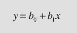
4.3 Classical Linear Regression Analysis and Prediction
Linear regression o ers another way of describing the relationship between
the two variables x and y. Whereas Pearson’s correlation coe cient provides
only a rough measure of a linear trend, linear models obtained by regres-
sion analysis allow the prediction of arbitrary y values for any given value
of x within the data range. Statistical testing of the signi cance of the linear
model provides some insights into the accuracy of these predictions.
Classical regression assumes that y responds to x, and that the entire
dispersion in the data set is in the y-value (Fig. 4.4). is means that x is
then the independent, regressor, or predictor variable. e values of x are
de ned by the experimenter and are o en regarded as being free of errors.
An example is the location x within a sediment core of a clay sample from
which the variable y has been measured. e dependent variable y contains
errors as its magnitude cannot be determined accurately. Linear regression
minimizes the deviations Δy between the data points xy and the value y
predicted by the best- t line y=b
0
+b
1
x using a least-squares criterion. e
basic equation for a general linear model is
where b
0
and b
1
are the regression coe cients. e value of b
0
is the inter-
cept with the y-axis and b
1
is the slope of the line. e squared sum of the
4.3 CLASSICAL LINEAR REGRESSION ANALYSIS AND PREDICTION 89
4 BIVARIATE STATISTICS
y-intercept b
0
y
Regression line
Regression line:
y = b
0
+ b
1
x
i-th data point (x
i
,y
i
)
Δy
Δx
Δx=1
Δy=b
1
02468
0
1
2
3
4
5
6
7
1
3
5
7
x
Linear Regression
Fig. 4.4 Linear regression. Whereas classical regression minimizes the Δy deviations,
reduced major axis regression minimizes the triangular area 0.5*(ΔxΔy) between the data
points and the regression line, where Δx and Δy are the distances between the predicted
and the true x and y values. e intercept of the line with the y-axis is b
0
, and the slope is b
1
.
ese two parameters de ne the equation of the regression line.
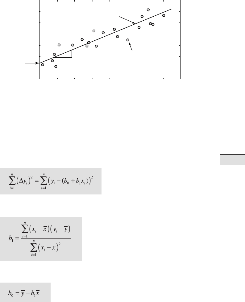
Δy deviations to be minimized is
Partial di erentiation of the right-hand term in the equation and setting it
to zero yields a simple equation for the regression coe cient b
1
:
e regression line passes through the data centroid de ned by the sample
means, and we can therefore compute the other regression coe cient b
0
,
using the univariate sample means and the slope b
1
computed earlier.
As an example, let us again load the synthetic age-depth data from the
90 4 BIVARIATE STATISTICS
le agedepth_1.txt. We can de ne two new variables, meters and age,
and generate a scatter plot of the data.
clear
agedepth = load('agedepth_1.txt');
meters = agedepth(:,1);
age = agedepth(:,2);
A signi cant linear trend in the bivariate scatter plot, together with a cor-
relation coe cient of more than r=0.9 suggests a strong linear dependence
between
meters and age. In geological terms, this implies that the sedi-
mentation rate was constant through time. We now try to t a linear model
to the data that will help us predict the age of the sediment at levels for which
we have no age data. e function
polyfit computes the coe cients of a
polynomial p(x) of a speci c degree that ts the data y in a least-squared
sense. In our example, we t a rst degree (linear) polynomial to the data.
p = polyfit(meters,age,1)
p =
5.5760 21.2480
Since we are working with synthetic data, we know the values for the slope
and the intercept with the y-axis. e estimated slope (5.5760) and the in-
tercept with the y-axis (21.2480) are in good agreement with the true values
of 5.6 and 20, respectively. Both the data and the tted line can be plotted
on the same graph.
plot(meters,age,'o'), hold on
plot(meters,p(1)*meters+p(2),'r'), hold off
Instead of using the equation for the regression line, we can also use the
function
polyval to calculate the y-values.
plot(meters,age,'o'), hold on
plot(meters,polyval(p,meters),'r'), hold off
Both, the functions polyfit and polyval are incorporated in the GUI
function
polytool.
polytool(meters,age)
e coe cients p(x) and the equation obtained by linear regression can
now be used to predict y-values for any given x-value. However, we can only
do this within the depth interval for which the linear model was tted, i.e.,

4.3 CLASSICAL LINEAR REGRESSION ANALYSIS AND PREDICTION 91
4 BIVARIATE STATISTICS
Depth in sediment (meters)
Age of sediment (kyrs)
Regression line
95% Error Bounds
95% Error Bounds
i-th data point
5101520
20
0
40
60
80
100
120
140
0
Bi
var
i
a
t
e
S
ca
tt
er
Fig. 4.5 e result of linear regression. e plot shows the original data points (circles), the
regression line (solid line), and the error bounds (dashed lines) of the regression. Note that
the error bounds are actually curved although they seem to be almost straight lines in the
example.
between 0 and 20 meters. As an example, the age of the sediment at a depth
of 17 meters is given by
polyval(p,17)
ans =
116.0405
is result suggests that the sediment at 17 meters depth has an age of ca.
116 kyrs. e goodness-of- t of the linear model can be determined by cal-
culating error bounds. ese are obtained by using an additional output pa-
rameter
s from polyfit as an input parameter for polyconf to calculate
the 95 % (
alpha=0.05) prediction intervals.
[p,s] = polyfit(meters,age,1);
[p_age,delta] = polyconf(p,meters,s,'alpha',0.05);
plot(meters,age,'o',meters,p_age,'g-',...
meters,p_age+delta,'r--',meters,p_age-delta,'r--')
axis([0 20 0 140]), grid on
xlabel('Depth in Sediment (meters)')
ylabel('Age of Sediment (kyrs)')
e variable delta provides an estimate for the standard deviation of the
92 4 BIVARIATE STATISTICS
error in predicting a future observation at x by p(x). Since the plot state-
ment does not t on one line, we use an ellipsis (three periods, i.e.,
...)
followed by return or enter to indicate that the statement continues on the
next line. e plot now shows the data points, and also the regression line
and the error bounds of the regression (Fig. 4.5). is graph already pro-
vides some valuable information on the quality of the result. However, in
many cases a better understanding of the validity of the model is required,
and more sophisticated methods for testing the con dence in the results are
therefore introduced in the following sections.
4.4 Analyzing the Residuals
When we compare how much the predicted values vary from the actual or
observed values, we are performing an analysis of the residuals. e statis-
tics of the residuals provide valuable information on the quality of a model
tted to the data. For instance, a signi cant trend in the residuals suggests
that the model does not fully describe the data. In such cases, a more com-
plex model such as a polynomial of a higher degree should be tted to the
data. Residuals are ideally purely random, i.e., Gaussian distributed with
zero mean. We therefore test the hypothesis that our residuals are Gaussian
distributed by visual inspection of the histogram and by employing a χ
2
-test,
as introduced in Chapter 3.
clear
agedepth = load('agedepth_1.txt');
meters = agedepth(:,1);
age = agedepth(:,2);
p = polyfit(meters,age,1);
res = age - polyval(p,meters);
Since plotting the residuals does not reveal any obvious pattern of behavior,
no more complex model than a straight line should be tted to the data.
plot(meters,res,'o')
An alternative way to plot the residuals is as a stem plot using stem.
subplot(2,1,1)
plot(meters,age,'o'), hold on
plot(meters,p(1)*meters+p(2),'r'), hold off

4.4 ANALYZING THE RESIDUALS 93
4 BIVARIATE STATISTICS
subplot(2,1,2)
stem(meters,res);
To explore the distribution of the residuals, we can choose six classes and
calculate the corresponding frequencies.
[n_exp,x] = hist(res,6)
n_exp =
4 6 5 7 5 3
x =
-12.7006 -7.3402 -1.9797 3.3807 8.7412 14.1016
By selecting bin centers in the locations de ned by the function hist, a
more practical set of classes can be de ned.
v = -25 : 8 : 20;
n_exp = hist(res,v);
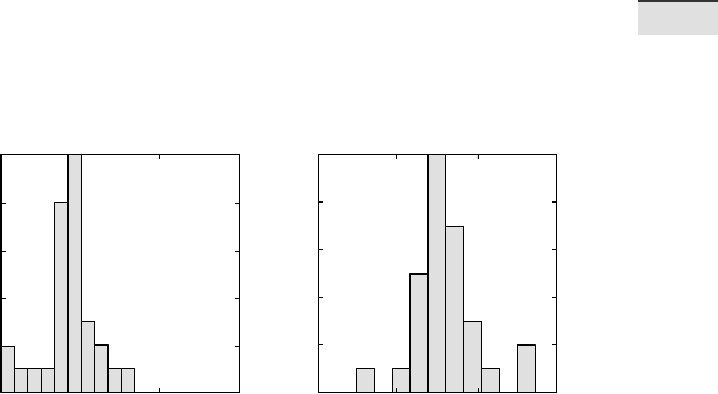
e mean and the standard deviation of the residuals are then computed,
and used to generate a theoretical distribution that can be compared with
the frequency distribution of the residuals. e mean is found to be close to
zero, and the standard deviation is 8.7922. e function
normpdf is used
to create the frequency distribution
n_syn similar to that in our example.
e theoretical distribution is scaled according to our original sample data
and displayed.
n_syn = normpdf(v,mean(res),std(res));
n_syn = n_syn ./ sum(n_syn);
n_syn = sum(n_exp) * n_syn;
e rst line normalizes n_syn to a total of one. e second command
scales
n_syn to the sum of n_exp. We can now plot both distributions for
comparison.
subplot(1,2,1), bar(v,n_syn,'r')
subplot(1,2,2), bar(v,n_exp,'b')
Visual inspection of the bar plots reveals similarities between the data sets.
Hence, the χ
2
-test can be used to test the hypothesis that the residuals fol-
low a Gaussian distribution.
chi2calc = sum((n_exp - n_syn) .^2 ./ n_syn)
chi2calc =
3.3747
94 4 BIVARIATE STATISTICS
e critical χ
2
can be calculated using chi2inv. e χ
2
test requires the
degrees of freedom Φ, which is the number of classes reduced by the num-
ber of variables and the number of parameters involved. In our example, we
de ned six classes, we tested the residuals for a Gaussian distribution with
two parameters (i.e., the mean and the standard deviation), testing at a 95 %
signi cance level, and the number of variables (i.e., the residuals) is one. e
degrees of freedom are therefore Φ=6–(2+1)=3.
chi2crit = chi2inv(0.95,3)
chi2crit =
7.8147
Since the critical χ
2
of 7.8147 is well above the measured χ
2
of 3.3747, it is
not possible to reject the null hypothesis. Hence, we can conclude that our
residuals follow a Gaussian distribution and that the bivariate data set is
therefore well described by the linear model.
4.5 Bootstrap Estimates of the Regression Coeffi cients
In this section we use the bootstrap method to obtain a better estimate of
the regression coe cients. As an example, we use the function
bootstrp
with 1000 samples (Fig. 4.6).
clear
agedepth = load('agedepth_1.txt');
meters = agedepth(:,1);
age = agedepth(:,2);
p = polyfit(meters,age,1);
p_bootstrp = bootstrp(1000,'polyfit',meters,age,1);
e statistic of the rst coe cient, i.e., the slope of the regression line is
hist(p_bootstrp(:,1),15)
mean(p_bootstrp(:,1))
std(p_bootstrp(:,1))
ans =
5.5644
ans =
0.3378

4.6 JACKKNIFE ESTIMATES OF THE REGRESSION COEFFICIENTS 95
4 BIVARIATE STATISTICS
Slope
Bootstrap Samples
Y−Axis Intercept
Bootstrap Samples
5.6±0.3
21.5±4.1
4567
0
50
100
150
200
010203040
0
50
100
150
1st Regression Coefficient 2st Regression Coefficient
ab
Fig. 4.6 Histogram of a, the rst (y-axis intercept of the regression line) and b, the second
(slope of the line) regression coe cient as estimated from bootstrap resampling. Whereas
the rst coe cient is well constrained, the second coe cient shows a broad scatter.
Because of variations in the random number generators used by bootstrp
results might vary slightly. e small standard deviation indicates that we
have an accurate estimate. In contrast, the statistic of the second parameter
shows a signi cant dispersion.
hist(p_bootstrp(:,2),15)
mean(p_bootstrp(:,2))
std(p_bootstrp(:,2))
ans =
21.5378
ans =
4.0745
e true values as used to simulate our data set are 5.6 for the slope and
20 for the intercept with the y-axis, whereas the corresponding coe cients
calculated using
polyfit were 4.0745 and 21.5378.
4.6 Jackknife Estimates of the Regression Coeffi cients
e jackknife method is a resampling technique that is similar to the boot-
strap method. From a sample with n data points, n subsamples with n–1
data points are taken. e parameters of interest, e. g., the regression coef-
96 4 BIVARIATE STATISTICS
cients, are calculated for each of the subsamples. e mean and dispersion
of the coe cients are computed. e disadvantage of this method is the
limited number of n subsamples. A jackknife estimate of the regression co-
e cients is therefore less precise than a bootstrap estimate.
e relevant code for the jackknife is easy to generate:
clear
agedepth = load('agedepth_1.txt');
meters = agedepth(:,1);
age = agedepth(:,2);
p = polyfit(meters,age,1);
for i = 1 : 30
j_meters = meters;
j_age = age;
j_meters(i) = [];
j_age(i) = [];
p(i,:) = polyfit(j_meters,j_age,1);
end
e jackknife for subsamples with n–1=29 data points can be obtained by a
simple
for loop. Within each iteration, the ith data point is deleted and re-
gression coe cients are calculated for the remaining data points. e mean
of the i subsamples gives an improved estimate of the regression coe cients.
As with the bootstrap result, the slope of the regression line ( rst coe cient)
is well de ned, whereas the intercept with the y-axis (second coe cient) has
a large uncertainty,
mean(p(:,1))
ans =
5.5757
compared to 5.56±0.34 calculated by the bootstrap method and
mean(p(:,2))
ans =
21.2528
compared to 21.54±4.07 from the bootstrap method. e true values, as
before, are 5.6 and 20. e histograms of the jackknife results from 30 sub-
samples (Fig. 4.7)
subplot(1,2,1), hist(p(:,1)), axis square
subplot(1,2,2), hist(p(:,2)), axis square
4.6 JACKKNIFE ESTIMATES OF THE REGRESSION COEFFICIENTS 97
4 BIVARIATE STATISTICS
Slope Y−Axis Intercept
ca. 5.6
ca. 21.2
Jackknife Samples
Jackknife Samples
5.4 5.6 5.8 6.0
18 20 22 24
0
2
4
6
8
10
0
2
4
6
8
10
1st Regression Coefficient 2st Regression Coefficient
ab
Fig. 4.7 Histogram of a, the rst (y-axis intercept of the regression line) and b, the second
(slope of the line) regression coe cient as estimated from jackknife resampling. Note that
the parameters are not as well de ned as those from bootstrapping.
do not display such clear distributions for the coe cients as the histograms
of the bootstrap estimates. As an alternative to the above method, MATLAB
provides the function
jackknife with which to perform a jackknife ex-
periment.
p = jackknife('polyfit',meters,age,1);
mean(p(:,1))
mean(p(:,2))
ans =
5.5757
ans =
21.2528
subplot(1,2,1), hist(p(:,1)), axis square
subplot(1,2,2), hist(p(:,2)), axis square
e results are identical to the ones obtained using the code introduced
above. We have seen therefore that resampling using either the jackknife
or the bootstrap method is a simple and valuable way to test the quality of
regression models. e next section introduces an alternative approach for
quality estimation, which is much more commonly used than the resam-
pling methods.