Trauth M.H., MATLAB® Recipes for Earth Sciences, Third edition

Подождите немного. Документ загружается.

98 4 BIVARIATE STATISTICS

4.7 Cross Validation

A third method to test the goodness-of- t of a regression is cross valida-

tion.  e regression line is computed by using n–1 data points.  e nth

data point is predicted and the discrepancy between the prediction and the

actual value is computed.  e mean of the discrepancies between the actual

and predicted values is subsequently determined.

In this example, the cross validation is computed for n=30 data points.

 e resulting 30 regression lines, each computed using n–1=29 data points,

display some dispersion in their slopes and y-axis intercepts.

clear

agedepth = load('agedepth_1.txt');

meters = agedepth(:,1);

age = agedepth(:,2);

p = polyfit(meters,age,1);

for i = 1 : 30

j_meters = meters;

j_age = age;

j_meters(i) = [];

j_age(i) = [];

p(i,:) = polyfit(j_meters,j_age,1);

plot(meters,polyval(p(i,:),meters),'r'), hold on

p_age(i) = polyval(p(i,:),meters(i));

p_error(i) = p_age(i) - age(i);

end

hold off

 e prediction error is – in the best case – Gaussian distributed with zero

mean.

mean(p_error)

ans =

0.0550

 e standard deviation is an unbiased mean of the deviations of the true

data points from the predicted straight line.

std(p_error)

ans =

9.6801

Cross validation gives valuable information on the goodness-of- t of the

4.8 REDUCED MAJOR AXIS REGRESSION 99

4 BIVARIATE STATISTICS

regression result, and can also be used also for quality control in other  elds,

such as those of temporal and spatial prediction (Chapters 5 and 7).

4.8 Reduced Major Axis Regression

In some cases, neither variable is manipulated and both can therefore be

considered to be independent. In these cases, several methods are available

to compute a best- t line that minimizes the distance from both x and y.

As an example, the method of reduced major axis (RMA) minimizes the

triangular area 0.5*(ΔxΔy) between the data points and the regression line,

where Δx and Δy are the distances between predicted and the true x and y

values (Fig. 4.4). Although this optimization appears to be complex, it can

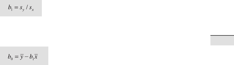
be shown that the  rst regression coe cient b

(the slope) is simply the ratio

of the standard deviations of y and x.

As with classical regression, the regression line passes through the data cen-

troid de ned by the sample mean. We can therefore compute the second

regression coe cient b

(the y-intercept),

using the univariate sample means and the slope b

computed earlier. Let us

again load the age-depth data from the  le agedepth_1.txt and de ne two

variables,

meters and age. It is assumed that both of the variables contain

errors and that the scatter of the data can be explained by dispersions of

meters and age.

clear

agedepth = load('agedepth_1.txt');

meters = agedepth(:,1);

age = agedepth(:,2);

 e above formula is used for computing the slope of the regression line b

p(1,1) = std(age)/std(meters)

p =

5.8286

100 4 BIVARIATE STATISTICS

 e second coe cient b

, i.e., the y-axis intercept, can therefore be com-

puted by

p(1,2) = mean(age) - p(1,1) * mean(meters)

p =

5.8286 18.7686

 e regression line can be plotted by

plot(meters,age,'o'), hold on

plot(meters,polyval(p,meters),'r'), hold off

 is linear  t di ers slightly from the line obtained from classical regres-

sion. Note that the regression line from RMA is not the bisector of the lines

produced by the x-y and y-x classical linear regression analyses, i.e., those

produced using either x or y as an independent variable while computing

the regression lines.

4.9 Curvilinear Regression

It is apparent from our previous analysis that a linear regression model pro-

vides a good way of describing the scaling properties of the data. However,

we may wish to check whether the data could be equally well described by

a polynomial  t of a higher degree, for instance by a second degree poly-

nomial:

To clear the workspace and reload the original data, we type

clear

agedepth = load('agedepth_1.txt');

meters = agedepth(:,1);

age = agedepth(:,2);

A second degree polynomial can then be  tted by using the function

polyfit.

p = polyfit(meters,age,2)

p =

-0.0544 6.6600 17.3246

4.9 CURVILINEAR REGRESSION 101

4 BIVARIATE STATISTICS

 e  rst coe cient is close to zero, i.e., has little in uence on predictions.

 e second and third coe cients are similar to those obtained by linear re-

gression. Plotting the data yields a curve that resembles a straight line.

plot(meters,age,'o'), hold on

plot(meters,polyval(p,meters),'r'), hold off

Let us compute and plot the error bounds obtained by using an optional sec-

ond output parameter from

polyfit as an input parameter to polyval.

[p,s] = polyfit(meters,age,2);

[p_age,delta] = polyval(p,meters,s);

As before, this code uses an interval of ± 2s, corresponding to a 95 % con -

dence interval. Using

polyfit not only yields the polynomial coe cients p,

but also a structure

s for use with polyval to obtain error bounds for the

predictions.  e variable

delta is an estimate of the standard deviation of

the prediction error of a future observation at

x by p(x). We then plot the

results:

plot(meters,age,'o',meters,p_age,'g-',...

meters,p_age+2*delta,'r', meters,p_age-2*delta,'r')

axis([0 20 0 140]), grid on

xlabel('Depth in Sediment (meters)')

ylabel('Age of Sediment (kyrs)')

We now use another synthetic data set that we generate using a quadratic

relationship between meters and age.

clear

rand('seed',40), randn('seed',40)

meters = 20 * rand(30,1);

age = 1.6 * meters.^2 - 1.1 * meters + 50;

age = age + 40.* randn(length(meters),1);

plot(meters,age,'o')

agedepth(:,1) = meters;

agedepth(:,2) = age;

agedepth = sortrows(agedepth,1);

save agedepth_2.txt agedepth -ascii

 e synthetic bivariate data set can be loaded from the  le agedepth_2.txt.

clear

agedepth = load('agedepth_2.txt');

102 4 BIVARIATE STATISTICS

Depth in sediment (meters)

Regression line

95% Error Bounds

i-th data point

02468101214161820

100

200

300

400

500

600

700

Age of sediment (kyrs

)

Curvilinear Regression

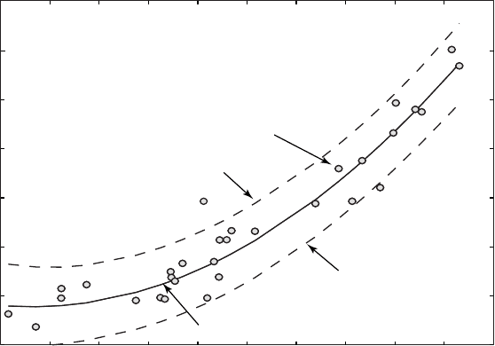
Fig. 4.8 Curvilinear regression from measurements of barium contents.  e plot shows the

original data points (circles), the regression line for a polynomial of degree n=2 (solid line),

and the error bounds (dashed lines) of the regression.

meters = agedepth(:,1);

age = agedepth(:,2);

plot(meters,age,'o')

Fitting a second order polynomial yields a convincing regression result.

p = polyfit(meters,age,2)

p =

1.6471 -4.2200 80.0314

As shown above, the true values for the three coe cients are +1.6, –1.1 and

+50, which means that there are some discrepancies between the true val-

ues and the coe cients estimated using

polyfit.  e regression curve

and the error bounds can be plotted by typing (Fig. 4.8)

plot(meters,age,'o'), hold on

plot(meters,polyval(p,meters),'r'), hold off

4.10 NONLINEAR AND WEIGHTED REGRESSION 103

4 BIVARIATE STATISTICS

[p,s] = polyfit(meters,age,2);

[p_age,delta] = polyval(p,meters,s);

plot(meters,age,'o',meters,p_age,'g',meters,...

p_age+2*delta,'r--',meters,p_age-2*delta,'r--')

axis([0 20 0 700]), grid on

xlabel('Depth in Sediment (meters)')

ylabel('Age of Sediment (kyrs)')

 e plot shows that the quadratic model for this data is a good one.  e

quality of the result could again be tested by exploring the residuals, by em-

ploying resampling schemes or by cross validation. Combining regression

analysis with one of these methods provides a powerful tool in bivariate

data analysis, whereas Pearson’s correlation coe cient should be used only

as a preliminary test for linear relationships.

4.10 Nonlinear and Weighted Regression

Many bivariate data in earth sciences follow a more complex trend than a

simple linear or curvilinear trend. Classic examples for nonlinear trends are

the exponential decay of radionuclides, or the exponential growth of algae

populations. In such cases, MATLAB provides various tools to  t nonlinear

models to the data. An easy-to-use routine to  t such models is nonlinear

regression using the function

nlinfit. To demonstrate the use of nlin-

fit we generate a bivariate data set where one variable is exponentially

correlated with a second variable. We  rst generate evenly-spaced values

between 0.1 and 3 in 0.1 intervals and add some Gaussian noise with a stan-

dard deviation of 0.2 to make the data unevenly spaced.  e resulting 30

data points are stored in the  rst column of the variable

data.

clear

randn('seed',0)

data(:,1) = 0.1 : 0.1 : 3;

data(:,1) = data(:,1) + 0.2*randn(size(data(:,1)));

Next, we can compute the second variable, which is the exponent of the  rst

variable multiplied by 0.2 and increased by 3. We again add Gaussian noise,

this time with a standard deviation of 0.5, to the data. Finally, we can sort

the data with respect to the  rst column and display the result.

data(:,2) = 3 + 0.2 * exp(data(:,1));

data(:,2) = data(:,2) + 0.5*randn(size(data(:,2)));

data = sortrows(data,1);

plot(data(:,1),data(:,2),'o')

104 4 BIVARIATE STATISTICS

xlabel('x-Axis'), ylabel('y-Axis')

Nonlinear regression aims to estimate the two coe cients of the expo-

nential function, i.e., the multiplier 0.2 and the summand 3.  e function

beta=nlinfit(data(:,1),data(:,2),fun,beta0) returns a vec-

tor

beta of coe cient estimates for a nonlinear regression of the re-

sponses in

data(:,2) on the predictors in data(:,1) using the model

speci ed by

fun. Here, fun is a function handle to a function of the form:

hat= modelfun(b,X), where b is a coe cient vector. A function handle

is passed in an argument list to other functions, which can then execute

the function using the handle. Constructing a function handle uses the at

sign,

@, before the function name.  e variable beta0 is a vector containing

initial values for the coe cients, and is the same length as

beta. We can

design a function handle model representing an exponential function with

variables an input variable

t and coe cients phi.  e initial values of beta

are

[0 0]. We can then use nlinfit to estimate the coe cients beta us-

ing the data, the model and the initial values.

model = @(phi,t)(phi(1)*exp(t) + phi(2));

beta0 = [0 0];

beta = nlinfit(data(:,1),data(:,2),model,beta0)

beta =

0.2006 3.0107

We can now use the resulting coe cients beta(1) and beta(2) to calcu-

late the function values

fittedcurve using the model and compare the

results with the original data.

fittedcurve = beta(1)*exp(data(:,1)) + beta(2);

plot(data(:,1),data(:,2),'o')

hold on

plot(data(:,1),fittedcurve,'r')

xlabel('x-Axis'), ylabel('y-Axis')

title('Unweighted Fit')

hold off

As we can see from the output of beta and the graph, the  tted red curve

describes the data fairly well. We can now also use

nlinfit to perform a

weighted regression. Let us assume that we know the one-sigma errors of

the values in

data(:,2). We can generate synthetic errors and store them

in the third column of

data.

data(:,3) = abs(randn(size(data(:,1))));

errorbar(data(:,1),data(:,2),data(:,3),'o')

xlabel('x-Axis'), ylabel('y-Axis')

4.10 NONLINEAR AND WEIGHTED REGRESSION 105

4 BIVARIATE STATISTICS

00.511.522.533.5

x−Axis

y−Axis

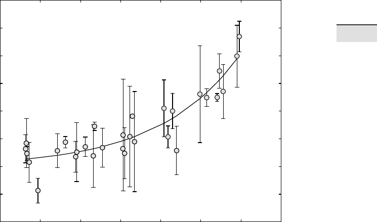
Weighted Fit

Fig. 4.9 Weighted regression from synthetic data.  e plot shows the original data points

(circles), the error bars of all data points, and the regression line for an exponential model

function (solid line).

We can now normalize the data points so that they are weighted by the in-

verse of the relative errors. We therefore normalize

data(:,3) so that the

total of all errors in

data(:,3) is one and store the normalized errors in

data(:,4).

data(:,4) = data(:,3)/sum(data(:,3));

To make a weighted  t, we  rst de ne weighted versions of the data

data(:,5) and the model function model, and then use nonlinear least

squares to make the  t.

data(:,5) = data(:,4).*data(:,2);

model = @(phi,t)(data(:,4).*(phi(1)*exp(t) + phi(2)));

beta0 = [0 0];

beta = nlinfit(data(:,1),data(:,5),model,beta0)

beta =

0.2045 2.9875

106 4 BIVARIATE STATISTICS

As before, nlinfit will compute weighted parameter estimates beta. We

again use the resulting coe cents

beta(1) and beta(2) to calculate the

function values

fittedcurve using the model and compare the results

with the original data.

fittedcurve = beta(1)*exp(data(:,1)) + beta(2);

errorbar(data(:,1),data(:,2),data(:,3),'o')

hold on

plot(data(:,1),fittedcurve,'r')

xlabel('x-Axis'), ylabel('y-Axis')

title('Weighted Fit')

hold off

Comparing the coe cients beta and the red curves from the weighted re-

gression with the previous results from the unweighted regression reveals

slightly di erent results (Fig. 4.9).

Recommended Reading

Alberède F (2002) Introduction to Geochemical Modeling. Cambridge University Press,

Cambridge

Davis JC (2002) Statistics and Data Analysis in Geology,  ird Edition. John Wiley and

Sons, New York

Draper NR, Smith, H (1998) Applied Regression Analysis. Wiley Series in Probability and

Statistics, John Wiley and Sons, New York

Efron B (1982)  e Jackknife, the Bootstrap, and Other Resampling Plans. Society of

Industrial and Applied Mathematics CBMS-NSF Monographs 38

Fisher RA (1922)  e Goodness of Fit of Regression Formulae, and the Distribution of

Regression Coe cients. Journal of the Royal Statistical Society 85:597–612

MacTavish JN, Malone PG, Wells TL (1968) RMAR; a Reduced Major Axis Regression

Program Designed for Paleontologic Data. Journal of Paleontology 42/4:1076–1078

Pearson K (1894–98) Mathematical Contributions to the  eory of Evolution, Part I to IV.

Philosophical Transactions of the Royal Society 185–191

 e Mathworks (2010) Statistics Toolbox 7 – User's Guide.  e MathWorks, Natick, MA

5 TIME-SERIES ANALYSIS

5 Time-Series Analysis

5.1 Introduction

Time-series analysis aims to investigate the temporal behavior of one of

several variables x(t). Examples include the investigation of long-term re-

cords of mountain upli , sea-level  uctuations, orbitally-induced insolation

variations and their in uence on the ice-age cycles, millenium-scale varia-

tions in the atmosphere-ocean system, the e ect of the El Niño/Southern

Oscillation on tropical rainfall and sedimentation (Fig. 5.1) and tidal in u-

ences on noble gas emissions from bore holes.  e temporal pattern of a

sequence of events can be random, clustered, cyclic or chaotic. Time-series

analysis provides various tools with which to detect these temporal pat-

terns. Understanding the underlying processes that produced the observed

data allows us to predict future values of the variable. We use the Signal

Processing and Wavelet Toolboxes, which contain all the necessary routines

for time-series analysis.

 e next section discusses signals in general and contains a technical

description of how to generate synthetic signals for time-series analysis

(Section 5.2).  e use of spectral analysis to detect cyclicities in a single

time series (auto-spectral analysis) and to determine the relationship be-

tween two time series as a function of frequency (cross-spectral analysis)

is then demonstrated in Sections 5.3 and 5.4. Since most time series in

earth sciences have uneven time intervals, various interpolation techniques

and subsequent methods of spectral analysis are introduced in Section 5.5.

Evolutionary power spectra to map changes in cyclicities through time are

demonstrated in Section 5.6. An alternative technique for analyzing uneven-

ly-spaced data is explained in Section 5.7. In the subsequent Section 5.8, the

very popular wavelet power spectrum is introduced, that has the capability

to map temporal variations in the spectra, in a similar way to the method

demonstrated in Section 5.6.  e chapter closes with an overview of nonlin-

ear techniques, in particular the method of recurrence plots (Section 5.9).

M.H. Trauth, MATLAB

Recipes for Earth Sciences, 3rd ed.,