Velten K. Mathematical Modeling and Simulation: Introduction for Scientists and Engineers

Подождите немного. Документ загружается.

3.6 Solution of ODE’s: Overview 155

The integral in this formula cannot be obtained in closed form. But since this

expression is needed so often in probability and statistics, it received its own name

andisreferredtoastheerror function erf (x) [105]. Using this function as a part

of the ‘‘well-known functions’’, many formulas can be written in closed form in

probability and statistics, which would not have been possible based on the usual

set of ‘‘well-known functions’’.

From a modeling point of view, it is desirable to have closed form solutions since

they tell us more about the system compared to numerical solutions. To see this,

consider Equation 3.25 again, the closed form solution of the body temperature

model, Equations 3.29 and 3.30:

T(t) = T

− (T

− T

) · e

−r · t

(3.106)

In this expression, the effects of the various model parameters on the resulting

temperature curve can be seen directly. In particular, it can be seen that the ambient

temperature, T

, as well as the initial temperature, T

, affect the temperature

essentially linear, while the rate parameter r has a strong nonlinear (exponential)

effect on the temperature pattern. To make this precise, Equation 3.106 could also

be used for a so-called sensitivity analysis, computing the derivatives of the solution

with respect to its parameters. The expression of T(t) in Equation 3.106 allows T to

be viewed as a multidimensional function

T(T

, T

, r, t) = T

− (T

− T

) ·e

−r · t

(3.107)

where we can take, for example, the derivative with respect to r as follows:

∂T(T

, T

, r, t)

∂r

= r · (T

− T

) ·e

−r · t

(3.108)

This is called the sensitivity of T with respect to r.OnthebasisofaTaylor

expansion, it can be used to estimate the effect of a change from r to r + r (r

being small) as

T(T

, T

, r + r, t) ≈ T(T

, T

, r, t) +

∂T(T

, T

, r, t)

∂r

· r (3.109)

A numerical solution of Equations 3.29 and 3.30, on the other hand, would give

us the temperature curve for any given set of parameters T

, T

, r similar to an

experimental data set, that is, it would provide us with a list of values (t

, T

), ...,(t

, T

) which we could then visualize, for example, using the plotting

capabilities of Maxima (Section 3.8.1). Obviously, we would not be able to see any

parameter effects based on such a list of data, or to compute sensitivities analytically

as above. The only way to analyze parameter effects using numerical solutions is to

compute this list of values (t

, T

), (t

, T

), ...,(t

, T

) for several different values of

a parameter, and then to see how it changes. Alternatively, parameter sensitivities

could also be computed using appropriate numerical procedures. However, you

156 3 Mechanistic Models I: ODEs

would have these numerically computed sensitivities only at some particular points,

and it is of course better and gives you more information on the system if you have

a general formula like Equation 3.108. In situations where you cannot get a closed

form solution for a mathematical model, it may, thus, be worthwhile to consider

a simpliﬁed version of the model that can be solved in terms of a closed form

solution. You will then have to trade off the advantages of the closed form solution

against the disadvantages of considering simpliﬁed versions of your model only.

3.7

Closed Form Solutions

Although mathematical models expressed as closed form solutions are very useful

as discussed above, an exhaustive survey of the methods that can be used to obtain

closed form solutions of ODEs would be beyond the scope of a ﬁrst introduction

to mathematical modeling techniques. This section is intended to give the reader a

ﬁrst idea of the topic based on a discussion of a few elementary methods that can

be applied to ﬁrst-order ODEs. For anything beyond this, the reader is referred to

the literature such as [100].

3.7.1

Right-hand Side Independent of the Independent Variable

Let us start our consideration of closed form solutions with the simplest ODE

discussed above (Equation 3.71 in Section 3.5.5):



= 0 (3.110)

3.7.1.1 General and Particular Solutions

Basically, we solved this equation ‘‘by observation’’, namely by the observation

that straight lines parallel to the x-axis have the property that the slope vanishes

everywhere as required by Equation 3.110. Here, ‘‘everywhere’’ of course refers

to the fact that we are talking about solutions of Equation 3.110 over the entire

set of real numbers. A more precise formulation of the problem imposed by

Equation 3.110 would be

(P1): Find a function T : R → R such that T



(x) = 0holdsforallx ∈ R.

In this formulation, it is implicitly assumed that the function T is differentiable

such that T



(t) can be computed everywhere in R. We could be more explicit (and

more precise) in this point using a speciﬁcation of the space of functions in which

we are looking for the solution:

(P2) Find a function T ∈ C

(R)suchthatT



(x) = 0holdsforallx ∈ R.

3.7 Closed Form Solutions 157

Here, C

(R) is the set of all functions having a continuous ﬁrst derivative on

R. In the theory of differential equations, particularly in the theory of PDEs, a

precise consideration of the function spaces where the solutions of differential

equations are sought for is of great importance. These functions spaces are used as

a subtle measure of the differentiability or smoothness of functions. For example,

the theory of PDEs leads to the so-called Sobolev spaces that involve functions that

are not differentiable in the classical sense, but are, nevertheless, used to solve

differential equations involving derivatives (see Section 4.7.1 for more details). All

this, however, is beyond the scope of this ﬁrst introduction into mathematical

modeling techniques.

Note 3.7.1 (Notation convention) If we write down an equation such as

Equation 3.110 with no further comments and restrictions, it will be under-

stood that we are looking for a sufﬁciently differentiable function on all of R.If

there can be no misunderstanding, a formulation like Equation 3.110 will always

be preferred to alternative formulations such as (P1) or (P2) above.

Now let us go back to the problem of solving Equation 3.110. As discussed in

Section 3.5.5, the observation ‘‘straight lines parallel to the x axis solve Equation

3.110’’ leads to the following expression for the solution of Equation 3.110:

T(x) = c, c ∈ R (3.111)

This is called the general solution of Equation 3.110 since it was derived from that

equation without any extra (initial or boundary) conditions. Note that Equation 3.111

describes an entire family of solutions parameterized by c,thatis,foreveryc ∈ R

we get a particular solution of Equation 3.110 from the general solution (Equation

3.111). General solutions of differential equations are typically described by such

families of solutions that are parameterized by certain parameters. We will see

several more examples of general solutions below. As explained before, initial or

boundary conditions are the appropriate means to pick out one particular solution

from the general solution, that is, to ﬁx one particular value of c inthecaseof

Equation 3.111.

3.7.1.2 Solution by Integration

To say that we solved Equation 3.110 ‘‘by observation’’ is of course a very un-

satisfactory statement, which cannot be generalized to more complex equations

We obviously need computational procedures to obtain the solution. Regarding

Equation 3.110, we can simply integrate the equation (corresponding to using the

fundamental theorem calculus) which then leads directly to the general solution

(Equation 3.111). The same technique can be applied to all ODEs having the

simple form



(x) = f (x) (3.112)

158 3 Mechanistic Models I: ODEs

Assuming that f (x) is deﬁned and continuous on some interval [a, b], the

fundamental theorem calculus states [17] that

T(x) =



f (s) ds + c, c ∈ R, x ∈ [a, b] (3.113)

solves Equation 3.112. Since f is assumed to be continuous (Deﬁnition 3.5.1), we

know that the integral on the right-hand side of Equation 3.113 can be evaluated. Of

course, continuity of the right-hand side of an ODE was required in Deﬁnition 3.5.1

exactly for this reason, that is, to make sure that solution formulas such as Equation

3.113 make good sense. In the sense explained above, Equation 3.113 is the general

solution of Equation 3.112, and it is again a family of solutions parameterized by

c ∈ R. As before, particular solutions of Equation 3.112 are obtained by imposing

an initial condition. From Equation 3.113, you see that T(0) = c, which shows that

c is the initial value of T at x = 0, so you see that the value of c (and hence a

particular case of Equation 3.113) is indeed ﬁxed if you impose an initial condition.

3.7.1.3 Using Computer Algebra Software

You will agree that what we did so far did not really involve a great deal of deep

mathematics. Anyone with that basic mathematical education assumed in this

book will do all this easily by hand. Nevertheless, we have a good starting point

here to see how a computer algebra software such as Maxima can be used to solve

ODEs (Appendix C). As explained before, the Maxima procedures used in this

book translate easily into very similar corresponding procedures in other computer

algebra software that you might prefer. Let us begin with Equation 3.110. In terms

of Maxima, this equation is written as

´diff(T,x)=0;

(3.114)

Comparing this with Equation 3.110, you see that the operator ‘diff(.,x)

designates differentiation with respect to x. To work with this equation in Maxima,

it should be stored in a variable like this:

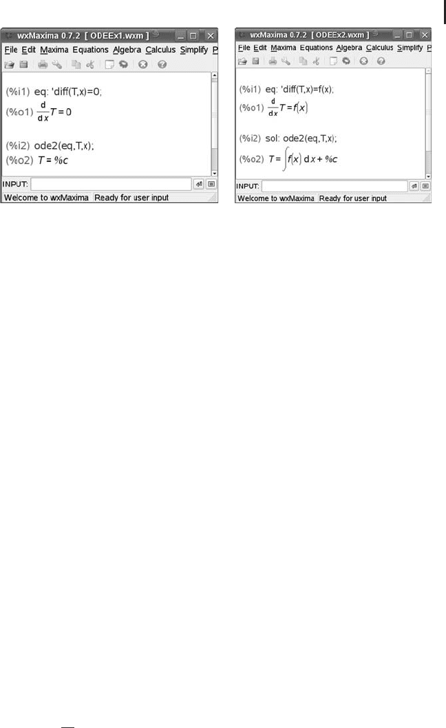
eq: ´diff(T,x)=0;

(3.115)

Now you can solve the ODE using the ode2 command as follows:

ode2(eq,T,x);

(3.116)

This command instructs Maxima to solve the equation eq for the function

T which depends on the independent variable x. Figure 3.6a shows how this

procedure is realized in a wxMaxima session. As can be seen, Maxima writes the

result in the form

T=%c;

(3.117)

3.7 Closed Form Solutions 159

(

)(

)

Fig. 3.6 wxMaxima sessions solving (a) Equation 3.110 and (b) Equation 3.112.

which is Maxima’s way to express our general solution in Equation 3.111. As you

see, an expression such as

%c in a Maxima output denotes a constant that may

take on any value in R. This example is a part of the book software (see the ﬁle

ODEEx1.mac).

Figure 3.6b shows an analogous wxMaxima session for the solution of Equation

3.112. As the ﬁgure shows, Maxima writes the solution as

T =



f (x) dx + %c (3.118)

This corresponds to the general solution derived above in Equation 3.113. Again,

%c is an arbitrary real constant. Maxima expresses the integral in its indeﬁnite

form, which means that appropriate integration limits should be inserted by the

‘‘user’’ of this solution formula similar to those used in Equation 3.113. Note that

the x in Equation 3.118 is just an integration variable, but it is not the independent

variable on which the solution function T depends. Equation 3.113 clariﬁes this

point. Maxima’s notation may be considered a little bit awkward here, but this is

the usual notation for indeﬁnite integrals, and it is not really a problem when you

read it carefully.

Of course, Maxima can easily evaluate the integral in Equation 3.118 when you

provide a concrete (integrable) expression for f (x). For example, solving



(x) = x

(3.119)

instead of Equation 3.112 and using the same procedure as above, Maxima produces

the correct general solution

T =

+ %c (3.120)

160 3 Mechanistic Models I: ODEs

which corresponds to

T(x) =

+ c, c ∈ R (3.121)

in the usual mathematical notation (see ODEEx3.mac in the book software).

Note 3.7.2 (Computer algebra software solves ODEs) Computer algebra soft-

ware such as Maxima can be used to solve ODEs either in closed form or

numerically. Closed form solutions are obtained in Maxima using the

ode2 com-

mand (and/or the

ic1, ic2,anddesolve commands, see below) and numerical

solutions using the

rk command (see below).

3.7.1.4 Imposing Initial Conditions

So far we have seen how general solutions of ODEs can be computed using

Maxima. The next step is to pick out particular solutions using initial or boundary

conditions. Maxima provides the command

ic1 to impose initial conditions

in ﬁrst-order equations and a corresponding command

ic2 for second-order

equations. Let us look at the following initial value problem for Equation 3.119:



(x) = x

(3.122)

T(0) = 1 (3.123)

Using the general solution, Equation 3.113, it is easily seen that the initial

condition, Equation 3.123, leads us to c = 1 such that the solution of Equations

3.122 and 3.123 is

T(x) =

+ 1 (3.124)

In Maxima, this is obtained using the following lines of code (see ODEEx4.mac

in the book software):

1: eq: ´diff(T,x)=xˆ2;

2: sol: ode2(eq,T,x);

3: ic1(sol,x=0,T=1);

(3.125)

As before, the ‘‘1:’’, ‘‘2:’’, ‘‘3:’’ at the beginning of each line are not a part of

the code, but just line numbers which we will use for reference. The ﬁrst two lines

of this code produce the general solution (3.120) following the same procedure as

above, the only difference being that the general solution is stored in the variable

sol in line 2 for further usage. Line 3 instructs Maxima to take the general solution

stored in

sol, and then to set T = 1atx = 0, that is, to impose the initial condition

(3.123). Maxima writes the results of these lines as

T =

+ 3

(3.126)

which is the same as Equation 3.124 as required. If you want Maxima to produce

this result exactly in the better readable form of Equation 3.124, you can use the

3.7 Closed Form Solutions 161

expand command as follows:

1: eq: ´diff(T,x)=xˆ2;

2: sol: ode2(eq,T,x);

3: ic1(sol,x=0,T=1);

4: expand(%);

(3.127)

The expand command in line 4 is applied to ‘‘%’’. Here, ‘‘%’’ refers to the last

output produced by Maxima, which is the result of the

ic1 command in line 3.

This means that the

expand command in line 4 is applied to the solution of the

initial value problem (Equation 3.126). Another way to achieve the same result

would have been to store the result of line 3 in a variable, and then to apply the

expand command to that variable, as it was done in the previous lines of the code.

As you can read in the Maxima manual, the

expand command splits numerators

of rational expressions that are sums into their respective terms. In this case, this

leads us exactly from Equation 3.126 to 3.124 as required.

As it was discussed above, the general form of Equation 3.122 is this:



(x) = f (x) (3.128)

We have seen that Equation 3.118 is the general solution of this equation. This

means that solving this kind of ODEs amounts to the problem of integrating f (x).

This can be done using the procedure described above, that is, by treating Equation

3.128 as before. On the other hand, we could also have used a direct integration

of f (x)basedonMaxima’s command for the integration of functions:

integrate.

For example, to solve Equation 3.119, we could have used the simple command

integrate(xˆ2,x);

(3.129)

See ODEEx5.mac in the book software. Maxima writes the result in the form

(3.130)

Except for the fact that Maxima skips the integration constant here, we are back

at the general solution (Equation 3.113) of Equation 3.119. In cases where the

integral of the right-hand side of Equation 3.128 cannot be obtained in closed form,

the numerical integration procedures of Maxima can be used (see e.g. Maxima’s

QUADPACK package).

3.7.2

Separation of Variables

The simple differential equations considered so far provided us with a nice

playground for testing Maxima procedures, but differential equations of this kind

would of course hardly justify the use of computer algebra software. So let us go on

162 3 Mechanistic Models I: ODEs

now toward more sophisticated ODEs. Solving ODEs becomes interesting when

the right-hand side depends on y. The simplest ODE of this kind is this:



= y (3.131)

You remember that this was the ﬁrst ODE considered above in Section 3.3.

Again, we solved it ‘‘by observation’’, observing that Equation 3.131 requires

the unknown function to coincide with its derivative, which is satisﬁed by the

exponential function:

y(x) = c · e

, c ∈ R (3.132)

Equation 3.132 is the general solution of Equation 3.131. Of course, it is again

quite unsatisfactory that we got this only ‘‘by observation’’. We saw above that

the fundamental theorem of calculus can be used to solve ODEs having the form

Equation 3.112. Obviously, this cannot be applied to Equation 3.131. Are there any

computational procedures that can be applied to this equation? Let us hear what

Maxima says to this question. First of all, let us note that Maxima solves Equation

3.131 using the above procedure (see

ODEEx7.mac in the book software):

1: eq: ´diff(y,x)=y;

2: ode2(eq,y,x);

(3.133)

If you execute this code, Maxima expresses the solution as

y = %c%e

(3.134)

As before, %c designates an arbitrary constant. You may be puzzled by the second

percentsign,butthisisjustapartoftheEulernumberwhichMaxima writes as

%e.

So we see that Maxima correctly reproduces Equation 3.132, the general solution of

Equation 3.131. But remember that we were looking for a computational procedure

to solve Equation 3.131. So far we have just seen that Maxima can do it somehow.

To understand the computational rule used by Maxima, consider the following

generalization of Equation 3.131:



= f (x) · g(y) (3.135)

Obviously, Equation 3.131 is obtained from this by setting g(y) = y and f (x) = 1.

Equation 3.128 is also obtained as a special case from Equation 3.135 if we set

g(y) = 1. Now confronting Maxima with Equation 3.135, it must tell us the rule

which it uses since it will of course be unable to compute a detailed solution like

Equation 3.134 without a speciﬁcation of f (x)andg(y). To solve Equation 3.135,

the following code can be used (see

ODEEx8.mac in the book software):

1: eq: ´diff(y,x)=f(x)*g(y);

2: ode2(eq,y,x);

(3.136)

3.7 Closed Form Solutions 163

Maxima writes the result as follows:



g(y)

dy =



f (x) dx + %c (3.137)

This leads to the following note:

Note 3.7.3 (Separation of variables method) The solution y(x)ofEquation

3.135 satisﬁes



g(y)

dy =



f (x) dx + c, c ∈ R (3.138)

In the literature, this method is often formally justiﬁed by writing Equation

3.135 as

= f (x) · g(y) (3.139)

that is, by using Leibniz’s notation of the derivative, and then by ‘‘separating the

variables’’ on different sides of the equation as

g(y)

= f (x) dx (3.140)

assuming g(y) = 0, of course. Then, a formal integration of the last equation yields

the separation of variables method (Equation 3.138).

Note that if g(y) = 1, that is, in the case of Equation 3.128, we get

y =



1 dy =



f (x) dx + c, c ∈ R (3.141)

which means that we correctly get the general solution (3.113), which turns out

to be a special case of Equation 3.138. Now let us look at Equation 3.131, which

is obtained by setting g(y) = y and f (x) = 1 in Equation 3.135 as observed above.

Using this in Equation 3.138 and assuming y = 0, we get



dy =



1 dx + c, c ∈ R (3.142)

ln|y|=x + c, c ∈ R (3.143)

which leads by exponentiation to

|y|=e

x+c

, c ∈ R (3.144)

164 3 Mechanistic Models I: ODEs

or, resolving the absolute value and denoting sgn(y) · e

as a new constant c,

y = c · e

, c ∈ R\{0} (3.145)

Since y = 0 is another obvious solution of Equation 3.131, the general solution

canbewrittenas

y = c · e

, c ∈ R (3.146)

3.7.2.1 Application to the Body Temperature Model

As another example application of Equation 3.138, let us derive the solution of the

body temperature model (Equation 3.29 in Section 3.4.1):



(t) = r · (T

− T(t)) (3.147)

To apply Equation 3.138, we ﬁrst need to write the right-hand side of the last

equation in the form of Equation 3.135, that is,



= f (t) · g(T) (3.148)

Since Equation 3.147 is an autonomous equation, we can set

f (t) = 1 (3.149)

g(T) = r · (T

− T) (3.150)

Equation 3.138 now tells us that the solution is obtained from



r · (T

− T)

dT =



1 dx + c, c ∈ R (3.151)

Using the substitution z = T

− T(t) in this integral and an analogous argu-

mentation as above in Equations 3.142–3.146 the general solution is obtained as

T(t) = T

+ c · e

−rt

, c ∈ R (3.152)

Applying the initial condition

T(0) = T

(3.153)

one obtains

c = T

− T

(3.154)

and hence

T(t) = T

+ (T

− T

) ·e

−r · t

(3.155)

which is the solution obtained ‘‘by observation’’ in Section 3.4.1 (Equation 3.25).