Wai-Fah Chen.The Civil Engineering Handbook

Подождите немного. Документ загружается.

29-20 The Civil Engineering Handbook, Second Edition

29.25). With commonly available software tools, such as spreadsheets, Eq. (29.28) can be readily solved

for one variable if the remaining two variables are known. The Moody diagram also permits a graphical

solution. If Re and k

/D are known, the curve corresponding to the given k

/D is found, and the value of

f corresponding to the given Re on that curve can be immediately read.

For non-circular conduits or open-channel ﬂows, Eq. (29.28) (or the Moody diagram) can be used as

an approximation by substituting an effective diameter, D

eff

= 4R

for D, in determining the relative roughness

and the Reynolds number. In some problems, k

/D and/or Re may not be directly available, because the

discharge, Q, or the pipe diameter, D, is to be determined. For such problems, an iterative solution is

required, which can either be graphical using the Moody diagram or be accomplished via software.

Other traditional formulae describing ﬂow resistance in conduits, intended for use with water only,

are encountered in practice. The Chezy-Manning equation is used frequently in open-channel ﬂows and

is discussed more fully in that chapter. The Hazen-Williams equation is frequently used in the waterworks

industry, and is discussed in the chapter on hydraulic structures. These equations, while convenient,

approximate the more generally applicable Colebrook-White-type formulae only over a restricted range

of Re and k

/D. In practice, this may be compensated by judiciously adjusting the relevant empirical

coefﬁcients to particular situations.

Minor Losses

Head losses that are caused by localized disturbances to a ﬂow, such as by valves or pipe ﬁttings or in

open-channel transitions, are traditionally termed minor losses, and will be denoted by h

as distinct

from continuous head losses denoted previously by h

. Because they are not necessarily negligible, a more

precise term would be transition or local losses, because they occur at transitions from one fully developed

ﬂow to another. Being due to localized disturbances, they do not vary with the conduit length, but are

instead described by an overall head loss coefﬁcient, K

. The greater the ﬂow disturbance, the larger the

value of K

; for example, as a valve is gradually closed, the associated value of K

for the valve increases.

Similarly, K

for different pipe ﬁttings will vary somewhat with pipe size, decreasing with increasing pipe

size, since ﬁttings may not be geometrically similar for different pipe sizes. Values of K

for various types

of transitions are tabulated at the end of this chapter. An alternative treatment of minor losses replaces

the sources of the minor losses by equivalent lengths of pipes, which are often tabulated. In this way, the

problem is converted to one with entirely continuous losses, which may be computationally convenient.

The total head loss, h

, of Eq. (29.18) consists of contributions from both friction and transition losses:

(29.29)

In some problems with long pipe sections and few instances of minor losses, such that fL/D  K

, minor

losses may be indeed minor and therefore negligible.

Application 12: A Piping System with Minor Losses

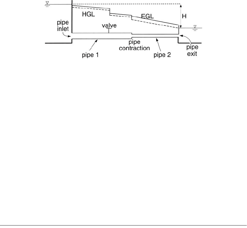
Consider a ﬂow between two reservoirs through the pipe system shown in Fig. 29.17. If the difference

in elevation between the two reservoirs is H, what is the discharge, Q? The energy equation between the

two free surfaces yields h

= H, since pressure and velocity heads are zero at the reservoir (control)

surfaces. The total head loss consists of friction losses in pipe 1 and pipe 2, as well as minor losses at the

entrance, the valve, the contraction, and the submerged exit:

hhh

Lfm

=+=

()

ÂÂ

mm m m

()

{}

()

{}

entrance valve contraction exit

Fundamentals of Hydraulics 29-21

where the subscripts refer to pipes 1 and 2. The minor loss coefﬁcients are obtained from tabulated values,

e.g., from Table 29.8 at the end of this chapter, (K

)

entrance

= 0.5. The friction factors, f

and f

, may differ

since Re and k

/D may differ in the two pipes. Because Q is not known, neither Re

nor Re

can be computed,

and hence neither f

nor f

can be directly determined from the Moody diagram: an iterative solution is

necessary if the Moody diagram is used. With an algebraic relationship for the friction factors, such as

Eq. (29.28), a simultaneous solution of the resulting nonlinear system of equations can be performed to

obtain Q. If an iterative graphical solution with the Moody diagram is undertaken, initial guesses of f

and

would be made, which would permit the evaluation of Q, and hence Re

and Re

could be estimated.

The friction factors corresponding to the thus estimated values of Re

and Re

are then checked for

consistency with the initial guesses for f

and f

; if they are in reasonable agreement, then a solution has

been found, otherwise the iterative procedure continues with additional guesses for f

and f

until consis-

tency is achieved. The HGL and EGL run parallel to each other in the two pipes; the distance between

them is however larger in pipe 2 because of the larger velocity head (due to the smaller pipe diameter).

The energy slope is constant for each pipe section, but will generally differ in the two pipe sections, with

the slope being larger in the case of the pipe with the smaller pipe due to larger velocity (S

µ V

). The

losses at transitions, shown as abrupt drops in the grade lines, are exaggerated for visual purposes.

29.8 Hydrodynamic Forces on Submerged Bodies

Bodies moving in ﬂuids or stationary bodies in a moving ﬂuid experience hydrodynamic forces in addition

to the hydrostatic forces discussed in Section 29.3. A net force in the direction of mean ﬂow is termed a

drag force, while a net force in the direction normal to the mean ﬂow is termed a lift force. These are

described in terms of dimensionless coefﬁcients of drag or lift, deﬁned as C

= F

/[(rU

/2)A

] and C

/[(rU

/2)A

], where the drag force, F

, and the lift force, F

, have been made dimensionless by the product

of the dynamic pressure, rU

/2, where U is the approach velocity (assumed constant) of the ﬂuid, and the

projected area, A

, of the body. In hydraulics, the drag force is usually of greater interest, as in the deter-

mination of the terminal velocity of sediment or of gas bubbles in the water column, or loads on structures.

The contribution due to skin friction drag, because of shear stresses on the body surface, is distinguished

from that due to form drag (also termed pressure drag), stemming from normal stresses (pressure) on the

body surface. At low Re (based on the relative velocity of body and ﬂuid) or in ﬂows around streamlined

bodies, skin friction drag will dominate, while in high Re ﬂows around bluff bodies, ﬂow separation will

occur and, with the formation of the low-pressure wake region, form drag will dominate.

The Standard Drag Curve

Theoretical results are available only for low Re ﬂows around bodies with simple geometrical shapes. For

steady ﬂow around solid spheres in a ﬂuid of inﬁnite extent and Re Æ 0, then C

= 24/Re, where Re 

UD/n, where U is the relative velocity of body in a ﬂuid with kinematic viscosity, n, and D is the diameter

of the sphere. In this so-called Stokes ﬂow regime, where Re <1, the terminal velocity of a solid sphere, w

FIGURE 29.17 A pipe system with minor (transitional) losses.

29-22 The Civil Engineering Handbook, Second Edition

i.e., the steady velocity it attains when falling under gravity in a stagnant ﬂuid of inﬁnite extent, is given

by w

= g(s

– s

/(18n), where s

and s

are respectively the speciﬁc gravities of the body and the ﬂuid.

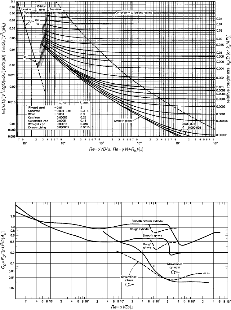
For larger Re and for more complicated geometries, empirical correlations for C

as a function of Re and

other factors such as relative roughness must be used. A standard drag curve (such as Fig. 29.23 at the

end of this chapter), which plots C

vs Re is available for common geometries, such as spheres or inﬁnitely

long circular cylinders. In these cases, C

exhibits a form of limited high Re similarity (see Sections 29.6

and 29.7) in the range, 10

< Re < 10,

where it attains an approximately constant value: C

ª 0.5 for

smooth spheres, and C

ª 1 for smooth inﬁnitely long circular cylinders. For high Re ﬂows around bluff

bodies without sharp edges to ﬁx the separation point, C

undergoes an abrupt decrease at a critical value

of Re because the separation point on the body moves downstream, resulting in a narrower low-pressure

wake region, and hence lower drag and smaller C

. For a smooth sphere or a smooth inﬁnitely long

cylinder, the critical value is observed to be ª 2 ¥ 10,

but surface roughness will decrease this critical value.

Application 13: Terminal Velocity of a Solid Sphere

Consider a metal sphere (density, r

, and diameter, D), falling under gravity in a ﬂuid (density, r, and

kinematic viscosity, n). When the sphere attains its terminal velocity, w

, its effective weight (including

hydrostatic buoyancy effects), g(r

– r)(pD

/6), is balanced by the drag force, F

= C

(rw

/2)A

, where

the projected area is taken to be A

= pD

/4, so that w

= . Since C

varies

with Re  w

D/n, and w

is unknown, the standard drag curve (in its graphical form) cannot be used

directly, and an iterative procedure is necessary to determine w

. As usual, the iterative solution might

begin with an initial guess for C

, from which a w

and a Re can be computed. A solution is obtained

when the computed Re is consistent with the guessed C

in agreeing with the standard drag curve.

29.9 Discharge Measurements

Discharge measurements are made for monitoring and control purposes. Measurement methods may be

divided into those for pipe and those for open-channel ﬂows. The following summarizes some results

for both types.

Pipe Flow Measurements

Traditional methods for measurements of discharge, Q, in a pipe of diameter, D, and cross-sectional area,

A, have depended on the production of a pressure difference, Dp, across a device constricting the ﬂow.

Foremost among such devices are various types of oriﬁce and Venturi meters, the basic theory of which

has been outlined in Appendixes 5 and 6.

In general, Q is related to the difference in piezometric head across the device, Dh, by

(29.30)

where A

is cross-sectional area of the contraction, and b = d/D, d being the diameter of the contracted

section. The discharge coefﬁcient, C

, may vary according to the device, the exact location of the pressure

taps where the measurements are made, b and Re. The head loss across the device, h

, is given as fraction

of measured differential pressure head.

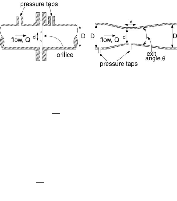
The common thin-plate oriﬁce meter is square-edged and concentric with the pipe (Fig. 29.18a). It is

used for clean ﬂuids and is inexpensive, but is associated with relatively high head loss. Miller (1989)

gives a correlation for C

for an oriﬁce with corner taps:

(29.31)

4g r

r§()1–[]D 3C

()§

Agh

()

=+ - +0 5959 0 0312 0 184

91 71

21 8

075

.. .

Fundamentals of Hydraulics 29-23

and a correlation for h

(29.32)

These correlations are valid for 0.2 < b < 0.75 and 10

< Re < 10

In comparison to oriﬁce meters, the Venturi meter (Fig. 29.18b) incurs low head losses, is suitable for

ﬂows with suspended solids, and exhibits less variation in performance characteristics. Disadvantages

include higher initial cost and the length and weight of the device. C

for a Venturi meter ranges from

0.975 to 0.995 (for Re > 5 ¥ 10

), while h

/Dh varies with the exit cone angle as (Miller, 1989)

(29.33)

Various other ﬂow meters are in use, and only a few are noted here. Elbow meters are based on the

pressure differential between the inner and the outer radius of the elbow. Attractive because of their low

cost, they tend to be less accurate than oriﬁce or Venturi meters, because of a relatively small pressure

differential. Rotameters or variable-area meters are based on the balance between the upward ﬂuid drag

on a ﬂoat located in an upwardly diverging tube and the weight of the ﬂoat. By the choice of ﬂoat and

tube divergence, the equilibrium position of the ﬂoat can be made linearly proportional to the ﬂow rate.

More recently developed non-mechanical devices include the electromagnetic ﬂow meter and the ultra-

sonic ﬂow meter. In the former, a voltage is induced between two electrodes that are located in the pipe

walls but in contact with the ﬂuid. The ﬂuid must be conductive, but can be multiphase. The output is

linearly proportional to Q, independent of Re, and insensitive to velocity proﬁle variations. Ultrasonic

ﬂow meters are based on the transmission and reception of acoustic signals, which can be related to the

ﬂow velocity. An attractive feature of some ultrasonic meters is that they can be clamped on to a pipe,

rather than being installed in place as is the case of most other devices.

Open-Channel Flow Measurements

Open-channel ﬂow measurements are typically based on measurements of ﬂow depth, which are then

correlated with discharge in head-discharge curves. The most common measurement structures may be

divided into weirs and critical-depth (Venturi) ﬂumes. Weirs are raised obstructions in a channel, with

the top of the obstruction being termed the crest. The streamwise extent of the weir may be short or

long, corresponding to sharp-crested and broad-crested weirs respectively. A critical-depth ﬂume is a

constriction built in an open channel, which causes the ﬂow to become critical (Fr = 1, see the discussion

FIGURE 29.18 Pipe ﬂow-measuring devices. (a) Thin-plate oriﬁce with corner pressure taps. (b) Venturi tube.

=- - -1024 052016

.. .bb b

=-+ =∞

0 436 0 83 0 59 15

0 218 0 42 0 38 7

...

bb q

29-24 The Civil Engineering Handbook, Second Edition

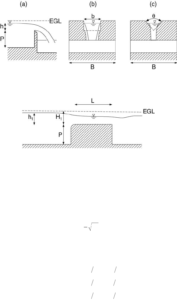
of critical ﬂows in the section on open-channel ﬂows) in, or near, the throat of the ﬂume. As shown in

Fig. 29.20a, the width of the channel will be denoted by B, the height of the weir crest above the channel

bottom is P, and the upstream elevation of the free surface relative to the weir crest is h. The ﬂuid is

assumed to be water, and viscous and surface tension effects are assumed negligible.

For a rectangular sharp-crested weir (Fig. 29.19b, see also Application 7), the head-discharge formula

may be expressed as

(29.34)

where b is the width of the weir opening, and C

is a discharge coefﬁcient that varies with b/B and h/P

as (Bos, 1989)

(29.35)

Equation (29.35) should give good results if h > 0.03 m, h/P < 2, P > 0.1 m, b > 0.15 m, and the water

surface level downstream of the weir should be at least 0.05 m below the crest. For contracted weirs

(b/B < 1), an alternative treatment of the effect of b/B uses an effective weir width, b

eff

, that is reduced

relative to the actual width, b. Further, the weir formula, Eq. (29.34), is often expressed as Q = C

weir

eff

3/2

where C

weir

is a weir coefﬁcient that varies with the system of units.

The triangular or V-notch weir (Fig. 29.19c) is often chosen when a wide range of discharges is expected,

since it is able to remain fully aerated at low discharges. The head-discharge formula for a triangular

opening with an included angle, q, may be expressed as

FIGURE 29.19 Open-channel discharge measurement structures. (a) Side view of a sharp-crested weir. (b) Front

view of a rectangular weir. (c) Front view of a triangular (V-notch) weir.

FIGURE 29.20 Broad-crested weir.

QC gbh

32/

ChPbB

hP bB

()

0 602 0 075 1

0 593 0 018 0 6

0 588 0 002 0 1

.. ,

.. , .

Fundamentals of Hydraulics 29-25

(29.36)

If h/P £ 0.4 and (h/B) tan(q/2) £ 0.2, then the discharge coefﬁcient, C

varies only slightly with q,

= 0.58 ± 0.01 for 25° < q < 90° (Bos, 1989). It is also recommended that h > 0.05 m, P > 0.45 m,

and B > 0.9 m.

Under ﬁeld conditions, where sharp-crested weirs may present maintenance problems, the broad-

crested weir (Fig. 29.20) provides a more robust structure. It relies on the establishment of critical ﬂow

(see the chapter of open-channel ﬂows for a discussion of critical ﬂows) over the weir crest. In order to

justify the neglect of frictional effects and the assumption of hydrostatic conditions over the weir, the

length of the weir, L, should satisfy 0.07 £ H

/L £ 0.5, where H

is the upstream total head referred to

elevation of the weir crest. The head-discharge formula may be expressed as

(29.37)

where C

is a discharge coefﬁcient, and C

is a coefﬁcient to account for a non-negligible upstream

velocity head (C

≥ 1, and C

= 1 if the approach velocity is neglected in which case H

= h; a graphical

correlation for C

is given in Bos, 1989). Bos (1989) recommends that C

= 0.93 + 0.10(H

/L).

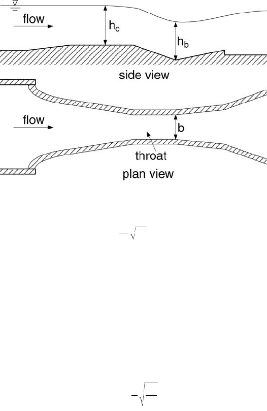
In situations where deposition of silt or other debris may pose a problem, a critical-depth ﬂume may

be more appropriate than a weir. Since it too is based on the establishment of critical ﬂow in the throat

of the ﬂume, its approximate theoretical analysis is essentially the same. The most common example is

the Parshall ﬂume (Fig. 29.21), which resembles a Venturi tube in having a converging section with a

level bottom, a throat section with a downward sloping bottom, and a diverging section with an upward

sloping bottom. The dimensioning of the Parshall ﬂume is standardized; as such the calibration curve

for each size (e.g., deﬁned by the throat width) is different, since the different sizes are not geometrically

similar. The head-discharge relation is typically expressed in terms of a piezometric head, h

, at a

prescribed location in the converging section, which is different for each size. This relationship is given

by Q = Kh

,where the exponent, m, ranges from 1.52 to 1.6, and the dimensional coefﬁcient, K, varies

with the size of the throat width, b

, with K ranging from 0.060 for b

= 1 in to 35.4 for b

= 50 ft. More

detailed information concerning K can be found in Bos (1989).

FIGURE 29.21 Critical-depth or Venturi ﬂume (Parshall type).

QC gh

52/

tanq

QCC

dB V

32/

29-26 The Civil Engineering Handbook, Second Edition

FIGURE 29.22 The Moody diagram. Adapted from Potter, M.C. and Wiggert, D.C. (1997). Mechanics of Fluids,

2nd ed., Prentice-Hall, Englewood Cliffs, NJ.

FIGURE 29.23 Drag coefﬁcients for ﬂow around various bluff bodies. Source: Potter, M.C. and Wiggart, D.C.

(1997). Mechanics of Fluids, 2nd ed., Prentice-Hall, Englewood Cliffs, NJ.

Fundamentals of Hydraulics 29-27

TA BLE 29.1 Physical Properties of Water in SI Units*

Te m p e r ature,

°F

Speciﬁc

We ig ht y,

lb/ft

Density

slugs/ft

Viscosity

m ¥ 10

lb·s/ft

Kinematic

Viscosity

n ¥ 10

Surface

Te nsion

s ¥ 10

lb/ft

Va po r

Pressure

psia

Va po r

Pressure

Head

/g,

Bulk

Modulus

of Elasticity

¥ 10

–3

psi

0 9.805 999.8 1.781 1.785 0.0756 0.61 0.06 2.02

5 9.807 1000.0 1.518 1.519 0.0749 0.87 0.09 2.06

10 9.804 999.7 1.307 1.306 0.0742 1.23 0.12 2.10

15 9.798 999.1 1.139 1.139 0.0735 1.70 0.17 2.14

20 9.789 998.2 1.002 1.003 0.0728 2.34 0.25 2.18

25 9.777 997.0 0.890 0.893 0.0720 3.17 0.33 2.22

30 9.764 995.7 0.798 0.800 0.0712 4.24 0.44 2.25

40 9.730 992.2 0.653 0.658 0.0696 7.38 0.76 2.28

50 9.689 988.0 0.547 0.553 0.0679 12.33 1.26 2.29

60 9.642 983.2 0.466 0.474 0.0662 19.92 2.03 2.28

70 9.589 977.8 0.404 0.413 0.0644 31.16 3.20 2.25

80 9.530 971.8 0.354 0.364 0.0626 47.34 4.96 2.20

90 9.466 965.3 0.315 0.326 0.0608 70.10 7.18 2.14

100 9.399 958.4 0.282 0.294 0.0589 101.33 10.33 2.07

*In this table and in the others to follow, if m ¥ 10

= 3.746 then m = 3.746 ¥ 10

–5

lb·s/ft

, etc. For example, at 80°F, s ¥

= 0.492 or s = 0.00492 lb/ft and E

¥ 10

–3

= 322 or E

= 322,000 psi.

From Daugherty, R.L., Franzini, J.B., and Finnemore, E.J. (1985) Fluid Mechanics with Engineering Applications, 8th ed.,

McGraw-Hill, New York. With permission.

TA BLE 29.2 Physical Properties of Water in English Units

Te m p e r ature,

°C

Speciﬁc

We ig ht y,

kN/m

Density

kg/m

Viscosity

m ¥ 10

N·s/m

Kinematic

Viscosity

n ¥ 10

Surface

Te nsion

N/m

Va po r

Pressure

kN/m

, abs

Va po r

Pressure

Head

/g,

Bulk

Modulus

of Elasticity

¥ 10

–6

kN/m

32 62.42 1.940 3.746 1.931 0.518 0.09 0.20 293

40 62.43 1.940 3.229 1.664 0.514 0.12 0.28 294

50 62.41 1.940 2.735 1.410 0.509 0.18 0.41 305

60 62.37 1.938 2.359 1.217 0.504 0.26 0.59 311

70 62.30 1.936 2.050 1.059 0.500 0.36 0.84 320

80 62.22 1.934 1.799 0.930 0.492 0.51 1.17 322

90 62.11 1.931 1.595 0.826 0.486 0.70 1.61 323

100 62.00 1.927 1.424 0.739 0.480 0.95 2.19 327

110 61.86 1.923 1.284 0.667 0.473 1.27 2.95 331

120 61.71 1.918 1.168 0.609 0.465 1.69 3.91 333

130 61.55 1.913 1.069 0.558 0.460 2.22 5.13 334

140 61.38 1.908 0.981 0.514 0.454 2.89 6.67 330

150 61.20 1.902 0.905 0.476 0.447 3.72 8.58 328

160 61.00 1.896 .838 0.442 0.441 4.74 10.95 326

170 60.80 1.890 0.780 0.413 0.433 5.99 13.83 322

180 60.58 1.883 0.726 0.385 0.426 7.51 17.33 318

190 60.36 1.876 0.678 0.362 0.419 9.34 21.55 313

200 60.12 1.868 0.637 0.341 0.412 11.52 26.59 308

212 59.83 1.860 0.593 0.319 0.404 14.70 33.90 300

From Daugherty, R.L., Franzini, J.B., and Finnemore, E.J. (1985) Fluid Mechanics with Engineering Applications, 8th ed.,

McGraw-Hill, New York. With permission.

29-28 The Civil Engineering Handbook, Second Edition

TA BLE 29.3 Physical Properties of Air at Standard Atmospheric Pressure in English Units

Te m p e r ature

Density

r ¥ 10

slugs/ft

Specifc Weight

g ¥ 10

lb/ft

Viscosity

m ¥ 10

lb·s/ft

Kinematic Viscosity

n ¥ 10

°F

°C

–40 –40.0 2.94 9.46 3.12 1.06

–20 –28.9 2.80 9.03 3.25 1.16

0 –17.8 2.68 8.62 3.38 1.26

10 –12.2 2.63 8.46 3.45 1.31

20 –6.7 2.57 8.27 3.50 1.36

30 –1.1 2.52 8.11 3.58 1.42

40 4.4 2.47 7.94 3.62 1.46

50 10.0 2.42 7.79 3.68 1.52

60 15.6 2.37 7.63 3.74 1.58

70 21.1 2.33 7.50 3.82 1.64

80 26.7 2.28 7.35 3.85 1.69

90 32.2 2.24 7.23 3.90 1.74

100 37.8 2.20 7.09 3.96 1.80

120 48.9 2.15 6.84 4.07 1.89

140 60.0 2.06 6.63 4.14 2.01

160 71.1 1.99 6.41 4.22 2.12

180 82.2 1.93 6.21 4.34 2.25

200 93.3 1.87 6.02 4.49 2.40

250 121.1 1.74 5.60 4.87 2.80

From Daugherty, R.L., Franzini, J.B., and Finnemore, E.J. (1985) Fluid Mechanics with Engi-

neering Applications, 8th ed., McGraw-Hill, New York. With permission.

TA BLE 29.4 The ICAO Standard Atmosphere in SI Units

Elevation Above

Sea Level,

Te m p e r ature,

°C

Absolute

Pressure,

kN/m

, abs

Speciﬁc

We ig ht y,

N/m

Density

kg/m

Speciﬁc

We ig ht y,

N·s/m

0 15.0 101.33 12.01 1.225 1.79

2 2.0 79.50 9.86 1.007 1.73

4 –4.5 60.12 8.02 0.909 1.66

6 –24.0 47.22 6.46 0.660 1.60

8 –36.9 35.65 5.14 0.526 1.53

10 –49.9 26.50 4.04 0.414 1.46

12 –56.5 19.40 3.05 0.312 1.42

14 –56.5 14.20 2.22 0.228 1.42

16 –56.5 10.35 1.62 0.166 1.42

18 –56.5 7.57 1.19 0.122 1.42

20 –56.5 5.53 0.87 0.089 1.42

25 –51.6 2.64 0.41 0.042 1.45

30 –40.2 1.20 0.18 0.018 1.51

From Daugherty, R.L., Franzini, J.B., and Finnemore, E.J. (1985) Fluid Mechanics

with Engineering Applications, 8th ed., McGraw-Hill, New York. With permission.

Fundamentals of Hydraulics 29-29

TA BLE 29.5 Physical Properties of Common Liquids at Standard Atmospheric Pressure in English Units

Liquid

Te m p e r ature

°F

Density

slug/ft

Speciﬁc

Gravity,

Viscosity

m ¥ 10

lb·s/ft

Surface

Te nsion

lb/ft

Va po r

Pressure

psia

Modulus of

Elasticity

psi

Benzene 68 1.74 0.90 1.4 0.002 1.48 150,000

Carbon tetrachloride 68 3.08 1.594 2.0 0.0018 1.76 160,000

Crude oil 68 1.66 0.86 15 0.002

Gasoline 68 1.32 068 0.62 …… 8.0

Glycerin 68 2.44 1.26 3100 0.004 0.000002 630,000

Hydrogen –430 0.14 0.072 0.043 0.0002 3.1

Kerosene 68 1.57 0.81 4.0 0.0017 0.46

Mercury 68 26.3 13.56 3.3 0.032 0.000025 3,800,000

Oxygen –320 2.34 1.21 0.58 0.001 3.1

SAE 10 oil 68 1.78 0.92 170 0.0025

SAE 30 oil 68 1.78 0.92 920 0.0024

Water681.936 1.00 2.1 0.005 0.34 300,000

From Daugherty, R.L., Franzini, J.B., and Finnemore, E.J. (1985) Fluid Mechanics with Engineering Applications,

8th ed., McGraw-Hill, New York. With permission.

TA BLE 29.6 Physical Properties of Common Liquids at Standard Atmospheric Pressure in SI Units

Liquid

Te m p e r ature

°F

Density

kg/m

Speciﬁc

Gravity,

Viscosity

m ¥ 10

N·s/m

Surface

Te nsion

N/m

Va po r

Pressure

kN/m

, abs

Modulus of

Elasticity

¥ 10

–6

N/m

Benzene 20 895 0.90 6.5 0.029 10.0 1030

Carbon tetrachloride 20 1588 1.59 9.7 0.026 12.1 1100

Crude oil 20 856 0.86 72 0.03

Gasoline 20 678 0.68 2.9 …… 55

Glycerin 20 1258 1.26 14,900 0.063 0.000014 4350

Hydrogen –257 72 0.072 0.21 0.003 21.4

Kerosene 20 808 0.81 19.2 0.025 3.20

Mercury 20 13,550 13.56 15.6 0.51 0.00017 26,200

Oxygen –195 1206 1.21 2.8 0.015 21.4

SAE 10 oil 20 918 0.92 820 0.037

SAE 30 oil 20 918 0.92 4400 0.036

Water20998 1.00 10.1 0.073 2.34 2070

From Daugherty, R.L., Franzini, J.B., and Finnemore, E.J. (1985) Fluid Mechanics with Engineering Applications,

8th ed., McGraw-Hill, New York. With permission.