Wai-Fah Chen.The Civil Engineering Handbook

Theory and Analysis of Structures 47-81

The terms in the ﬁrst column consist of the element forces q

1

through q

4

that result from displacement

d

1

= 1 when d

2

= d

3

= d

4

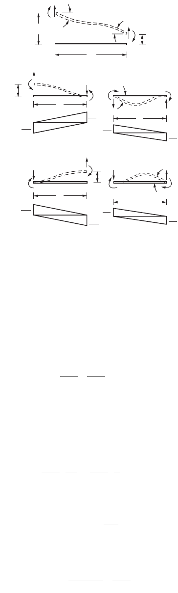
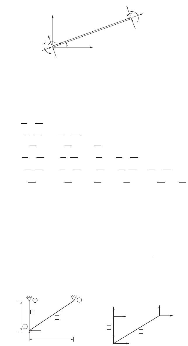
= 0. This means that a unit vertical displacement is imposed at the left end of

the member, while translation at the right end and rotation at both ends are prevented, as shown in

Fig. 47.74. The four member forces corresponding to this deformation can be obtained using the moment

area method.

The change in slope between the two ends of the member is zero, and the area of the M/EI diagram

between these points must therefore vanish. Hence

and

(47.135)

The moment of the M/EI diagram about the left end of the member is equal to unity. Hence

and in view of Eq. (47.135),

Finally, moment equilibrium of the member about the right end leads to

FIGURE 47.74 Beam element — stiffness matrix.

L

(a)

Flexural element

δ

1

δ

2

δ

4

δ

3

q

3

k

21

k

11

k

31

k

22

k

41

k

12

k

42

k

32

k

34

k

14

k

43

k

33

k

23

k

13

k

24

k

44

q

4

q

2

q

1

L

(c)(b)

(d) (e)

L

δ

1

= 1

δ

3

= 1

δ

2

= 1

δ

4

= 1

k

41

EI

k

42

EI

k

22

EI

k

24

EI

k

43

EI

k

23

EI

k

44

EI

k

21

EI

KL KL

41 21

2EI 2EI

0-=

KK

21 41

=

KL KL

41 21

2EI

2L

32EI

L

3

1

Ê

Ë

Á

ˆ

¯

˜

-

Ê

Ë

Á

ˆ

¯

˜

=

KK

EI

L

41 21

2

6

==

K

KK

11

21 41

=

+

=

L

12EI

L

3

47-82 The Civil Engineering Handbook, Second Edition

and from equilibrium in the vertical direction we obtain

The forces act in the directions indicated in Fig. 47.74b. To obtain the correct signs, one must compare

the forces with the positive directions deﬁned in Fig. 47.74a. Thus

The second column of the stiffness matrix is obtained by letting d

2

= 1 and setting the remaining three

displacements equal to zero, as indicated in Fig. 47.74c. The area of the M/EI diagram between the ends

of the member for this case is equal to unity, and hence

The moment of the M/EI diagram about the left end is zero, so that

Therefore, one obtains

From vertical equilibrium of the member,

and moment equilibrium about the right end of the member leads to

Comparison of the forces in Fig. 47.74c with the positive directions deﬁned in Fig. 47.74a indicates that

all the inﬂuence coefﬁcients except k

12

are positive. Thus

Using Figs. 47.74d and e, the inﬂuence coefﬁcients for the third and fourth columns can be obtained.

The results of these calculations lead to the following element stiffness matrix:

(47.136)

KK

EI

L

31 11

3

12

==

KK K K

11 21 31 41

==-=-=

12EI

L

,

6EI

L

,

12EI

L

,

6EI

L

3232

KL

EI

KL

EI

22 42

22

1-=

KL KL

22 42

2EI

L

32EI

2L

3

0

Ê

Ë

Á

ˆ

¯

˜

-

Ê

Ë

Á

ˆ

¯

˜

=

KK

22 42

==

4EI

L

,

2EI

L

KK

12 32

=

K

KK

L

EI

L

12

22 42

2

6

==

_

KKKK

12 22 32 42

=- = = =

6EI

L

,

4EI

L

,

6EI

L

,

2EI

L

22

q

EI

L

EI

L

EI

L

EI

L

EI

L

EI

L

EI

L

EI

L

EI

L

EI

L

EI

L

EI

L

EI

L

EI

L

EI

L

EI

L

1

2

3

4

3232

22

32 3 2

22

1

2

3

12

6126

64 6 2

12 6 12 6

62 6 4

È

Î

Í

˘

˚

˙

=

-- -

-

È

Î

Í

˘

˚

˙

d

44

È

Î

Í

˘

˚

˙

Theory and Analysis of Structures 47-83

Note that Eq. (47.135) deﬁnes the element stiffness matrix for a ﬂexural member with constant ﬂexural

rigidity EI.

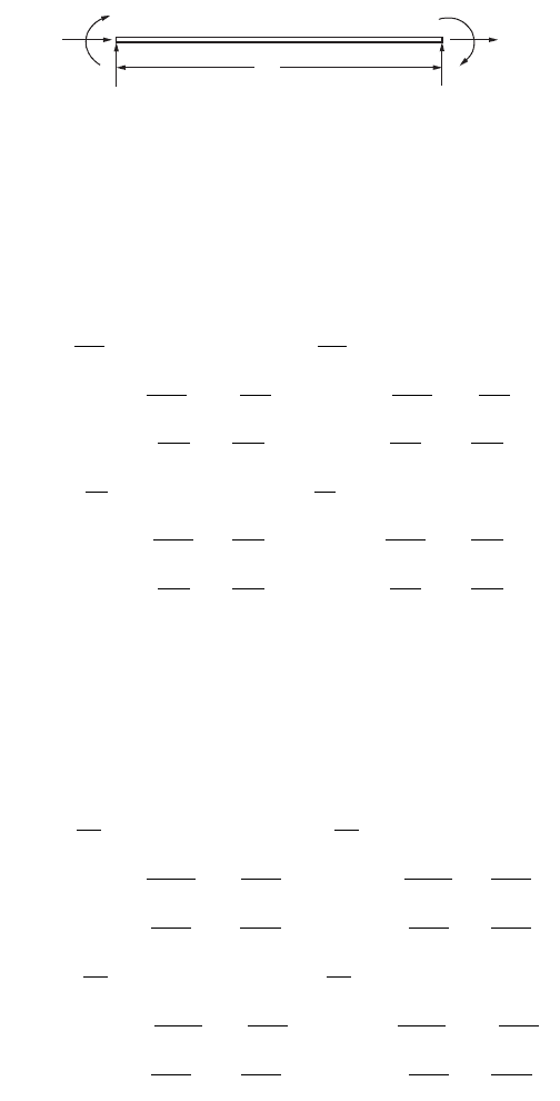
If the axial load in a frame member is also considered, the general form of an element stiffness matrix

for an element shown in Fig. 47.75 becomes

or

(47.137)

The member stiffness matrix can be written as

(47.138)

Structure Stiffness Matrix

Equation (47.137) has been expressed in terms of the coordinate system of the individual members. In

a structure consisting of many members there would be as many systems of coordinates as the number

of members. Before the internal actions in the members of the structure can be related, all forces and

deﬂections must be stated in terms of one single system of axes common to all — the global axes. The

transformation from element to global coordinates is carried out separately for each element, and the

resulting matrices are then combined to form the structure stiffness matrix. A separate transformation

matrix [T] is written for each element, and a relation of the form

FIGURE 47.75 Beam element with axial force.

L

E,A,I

q

1

q

2

q

3

q

4

q

5

q

6

q

EA

L

EA

L

EI

L

EI

L

EI

L

EI

L

EI

L

EI

L

EI

L

EI

L

EI

L

EI

L

EI

L

EI

L

EI

L

EI

L

EI

L

EI

1

2

3

4

5

6

32 32

22

32 3 2

2

00 00

0

12 6

0

12 6

0

64

0

62

00 00

0

12 6

0

12 6

0

62

È

Î

Í

˘

˚

˙

=

-

---

-

LL

EI

L

EI

L

0

64

2

1

2

3

4

5

6

È

Î

Í

˘

˚

˙

È

Î

Í

˘

˚

˙

d

qk

c

[]

=

[]

d

K

GJ

L

GJ

L

EI

L

EI

L

EI

L

EI

L

EI

L

EI

L

EI

L

EI

L

GJ

L

GJ

L

EI

L

EI

L

EI

L

EI

L

EI

L

EI

L

EI

L

EI

L

zz zz

zz z z

zz zz

=

-

-- -

-

È

Î

Í

0

00 00

0

12 6

0

12 6

0

64

0

62

00 00

0

12 6

0

12 6

0

62

0

64

32 32

22

22 3 2

22

ÍÍ

Í

˘

˚

˙

47-84 The Civil Engineering Handbook, Second Edition

(47.139)

is written in which [T]

n

deﬁnes the matrix relating the element deformations of element n to the structure

deformations at the ends of that particular element. The element and structure forces are related in the

same way as the corresponding deformations as

(47.140)

where [q]

n

contains the element forces for element n and [W]

n

contains the structure forces at the

extremities of the element. The transformation matrix [T]

n

can be used to transform element n from its

local coordinates to structure coordinates. We know, for an element n, that the force–deformation relation

is given as

Substituting for [q]

n

and [d]

n

from Eqs. (47.138) and (47.139), one obtains

or

(47.141)

[K]

n

is the stiffness matrix that transforms any element n from its local coordinate to structure coordi-

nates. In this way, each element is transformed individually from element coordinate to structure coor-

dinate, and the resulting matrices are combined to form the stiffness matrix for the entire structure.

For example, the member stiffness matrix [K]

n

in global coordinates for the truss member shown in

Fig. 47.76 is given as

(47.142)

in which l =cosf

m = sinf.

FIGURE 47.76 Grid member.

y

x

o

∆

i

∆

j

∆

k

∆

p

φ

d

[]

=

[][]

nnn

T D

qTW

nnn

[]

=

[][ ]

qk

nnn

[]

=

[][]

d

TW kT

nn nnn

[][ ]

=

[][][]

D

[] [][][][]

[][][][]

[][]

[] [][][]

WTkT

TkT

K

KTkT

nnnnn

n

T

nnn

nn

T

nn

=

-1

D

[]K

AE

L

i

j

k

n

=

--

È

Î

Í

˘

˚

˙

lm lm llm

lm m lm m

llmllm

lm m lm m

22

l

Theory and Analysis of Structures 47-85

To construct [K]

n

for a given member, it is necessary to have the values of l and m for the member.

In addition, the structure coordinates i, j, k, and l at the extremities of the member must be known.

The member stiffness matrix [K]

n

in structural coordinates for the ﬂexural member shown in Fig. 47.77

can be written as

(47.143)

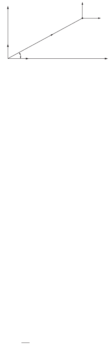
where l = cosf and m = sinf.

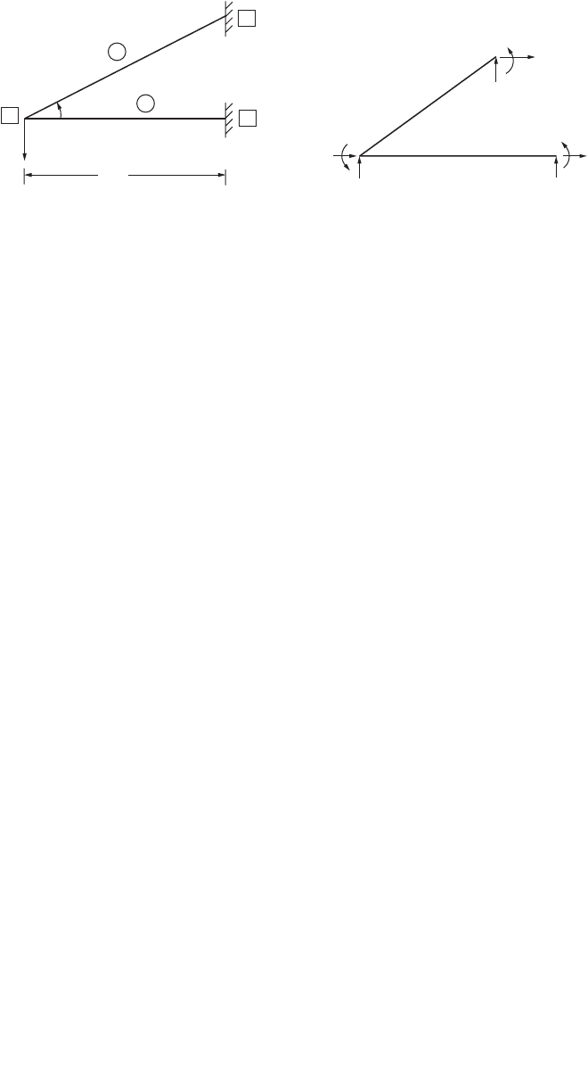
Example 47.9

Determine the displacement at the loaded point of the truss shown in Fig. 47.78a. Both members have

the same area of cross section: A = 3 and E = 30 ¥ 10

3

.

The details required to form the element stiffness matrix with reference to structure coordinates axes

are listed below (see Fig. 47.78b):

We now use these data in Eq. (47.142) to form [K]

n

for the two elements.

FIGURE 47.77 Flexural member in global coordinate.

Member Length fl mijkl

11090° 011234

2 18.9 32° 0.85 0.53 1256

FIGURE 47.78 Example 47.9.

X

Y

m

n

l

j

k

i

q

1

q

2

q

3

q

4

q

5

q

6

φ

K

AE

L

EI

L

AE

L

EI

L

AE

L

EI

L

symmetric

EI

L

EI

L

EI

L

AE

L

EI

L

AE

L

EI

L

EI

L

AE

L

EI

L

n

z

[]

=

+

-

Ê

Ë

Á

ˆ

¯

˜

+

-

Ê

Ë

Á

ˆ

¯

˜

-- -

Ê

Ë

Á

ˆ

¯

˜

Ê

Ë

Á

ˆ

¯

˜

+

0

12

12 12

6

4

0

12 12 6 12

00

22

3

22

3

22

332

22

3

lm

ml m l

ml

lm ml mlm

---

Ê

Ë

Á

ˆ

¯

˜

-+

Ê

Ë

Á

ˆ

¯

˜

-

Ê

Ë

Á

ˆ

¯

˜

-

Ê

Ë

Á

ˆ

¯

˜

+

Ê

Ë

Á

ˆ

¯

˜

Ê

Ë

Á

ˆ

¯

˜

-

È

Î

Í

ml m l l ml m l

ml ml

AE

L

EI

L

AE

L

EI

L

EI

L

AE

L

EI

L

AE

L

EI

L

EI

L

EI

L

EI

L

EI

L

EI

L

EI

L

zz

12 12

6

12 12

66

26

6

4

3

22

32 3

2

3

22 22

ÍÍ

Í

˘

˚

˙

7 k

9 k

16 ft

10 ft

3

1

2

1

5

1

2

3

4

6

2

1

47-86 The Civil Engineering Handbook, Second Edition

For member 1,

For member 2,

Combining the element stiffness matrices [K]

1

and [K]

2

, one obtains the structure stiffness matrix as follows:

The stiffness matrix can now be subdivided to determine the unknowns. Let us consider D

1

and D

2

, the

deﬂections at joint 2, which can be determined in view of D

3

= D

4

= D

5

= D

6

= 0 as follows:

or

Example 47.10

A simple triangular frame is loaded at the tip by 20 units of force, as shown in Fig. 47.80. Assemble the

structure stiffness matrix and determine the displacements at the loaded node.

Member Length A I fl m

1722.4 1037 0 1 0

2 101.8 3.4 2933 45° 0.707 0.707

AE

L

330

10

120

750

3

=

¥¥

=

[]

1234

0000

0 750 0 750

0000

0 750 0 750

1

2

3

4

1

K =

-

AE

L

330

10

18.9 12

397

3

=

¥¥

¥

=

[]

1256

286 179 286 179

179 111 179 111

286 179 286 179

179 111 179 111

1

2

5

6

2

K =

--

W

1

2

3

4

5

6

1

2

3

4

5

6

286 179 0 0 286 179

179 861 0 750 179 111

000000

0 750 0 750 0 0

286 179 0 0 286 179

179 111 0 0 179 111

È

Î

Í

˘

˚

˙

=

--

---

-

--

È

Î

Í

˘

˚

˙

È

Î

Í

D

ÍÍ

Í

˘

˚

˙

D

1

2

1

286 179

179 861

9

7

È

Î

Í

˘

˚

˙

=

È

Î

Í

˘

˚

˙

-

È

Î

Í

˘

˚

˙

-

D

1

2

0 042

0 0169

=

.

Theory and Analysis of Structures 47-87

For members 1 and 2 the stiffness matrices in structure coordinates can be written by making use of

Eq. (47.143):

and

Combining the element stiffness matrices [K]

1

and [K]

2

, one obtains the structure stiffness matrix as

follows:

FIGURE 47.79 Example 47.10.

2

1

2

3

6 ft

20 kips

45°

1

2

3

4

5

6

7

8

9

[]K

1

3

10

12 3 4 5 6

10 0 10 0

01 36 0136

0361728 0 36 864

1 0010 0

013601 36

036864 0 36 1728

1

2

3

4

5

6

=¥

-

-- -

-

Í

Î

Í

˙

˚

˙

[]K

2

3

10

12 3 78 9

10 3610 36

013601 36

36 36 3457 36 36 1728

10 36 10 36

01 3601 36

36 36 1728 36 36 3457

1

2

3

7

8

9

=¥

-- -

--

-

--

Í

Î

Í

˙

˚

˙

[]K =¥

-- - -

-

---

-

-- -

-

--

-

È

Î

Í

10

20 3610 01036

02720 136 0 1 36

36 72 5185 0 36 864 36 36 1728

1 0010 0 0 0 0

013601 36 0 0 0

036864 0 36 1728 0 0 0

10 36 0 0 0 1000 0 36

01 3600 00136

36 36 1728 0 0 0 36 36 3457

3

ÍÍ

Í

˘

˚

˙

1

2

3

4

5

6

7

8

9

47-88 The Civil Engineering Handbook, Second Edition

The deformations at joints 2 and 3 corresponding to D

5

to D

9

are zero, since joints 2 and 4 are restrained

in all directions. Canceling the rows and columns corresponding to zero deformations in the structure

stiffness matrix, one obtains the force–deformation relation for the structure:

Substituting for the applied load F

2

= –20, the deformations are given as

or

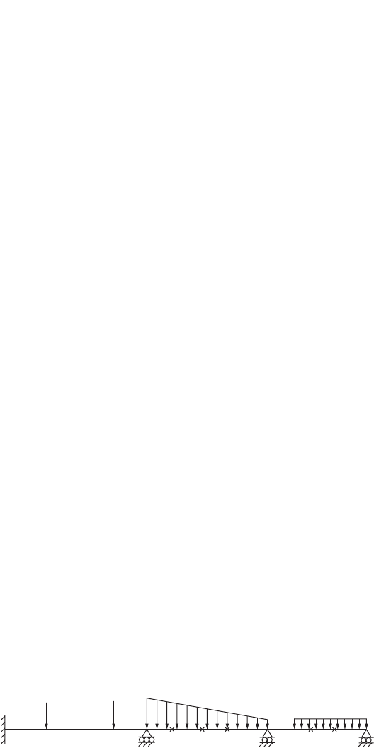
Loading between Nodes

The problems discussed so far have involved concentrated forces and moments applied only to nodes.

But real structures are subjected to distributed or concentrated loading between nodes, as shown in

Fig. 47.80. Loading may range from a few concentrated loads to an inﬁnite variety of uniform or

nonuniform distributed loads. The solution method of matrix analysis must be modiﬁed to account for

such load cases.

One way to treat such loads in the matrix analysis is to insert artiﬁcial nodes, such as p and q, as

shown in Fig. 47.80. The degrees of freedom corresponding to the additional nodes are added to the total

structure, and the necessary additional equations are written by considering the requirements of equi-

librium at these nodes. The internal member forces on each side of nodes p and q must equilibrate the

external loads applied at these points. In the case of distributed loads, suitable nodes such as l, m, and

n, shown in Fig. 47.80, are selected arbitrarily and the distributed loads are lumped as concentrated loads

at these nodes. The degrees of freedom corresponding to the arbitrary and real nodes are treated as

unknowns of the problem. There are different ways of obtaining equivalence between the lumped and

the distributed loading. In all cases the lumped loads must be statically equivalent to the distributed

loads they replace.

The method of introducing arbitrary nodes is not a very elegant procedure because the number of

unknown degrees of freedom make the solution procedure laborious. The approach that is of the most

general use with the displacement method is the one employing the related concepts of artiﬁcial joint

restraint, ﬁxed-end forces, and equivalent nodal loads.

FIGURE 47.80 Loading between nodes.

F

1

2

3

1

2

3

20 36

0272

36 72 5185

10

È

Î

Í

˘

˚

˙

=

-

È

Î

Í

˘

˚

˙

¥

È

Î

Í

˘

˚

˙

D

1

2

3

1

3

20 36

0272

36 72 5185

10

0

20

0

È

Î

Í

˘

˚

˙

=

-

È

Î

Í

˘

˚

˙

¥-

È

Î

Í

˘

˚

˙

-

D

1

2

3

666

23 334

0 370

10

È

Î

Í

˘

˚

˙

=-

È

Î

Í

˘

˚

˙

¥

.

lqp l m n m

Theory and Analysis of Structures 47-89

Semirigid End Connection

A rigid connection holds unchanged the original angles between interesting members; a simple connec-

tion allows the member end to rotate freely; a semirigid connection possesses a moment resistance

intermediate between those of the simple and rigid connections.

A simpliﬁed linear relationship between the moment M acting on the connection and the resulting

connection rotation y in the direction of M is assumed, giving

(47.144)

where EI and L are the ﬂexural rigidity and length of the member, respectively. The nondimension

quantity R, which is a measure of the degree of rigidity of the connection, is called the rigidity index.

For a simple connection, R is zero; for a rigid connection, R is inﬁnity. Considering the semirigidity of

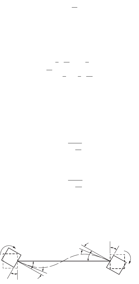
joints, the member ﬂexibility matrix for ﬂexure is derived as

(47.145)

or

(47.146)

where f

1

and f

2

are as shown in Fig. 47.81.

For convenience, two parameters are introduced as follows

and

where p

1

and p

2

are called the ﬁxity factors. For hinged connections, both the ﬁxity factors, p, and the

rigidity index, R, are zero, but for rigid connections, the ﬁxity factor is 1 and the rigidity index is inﬁnity.

Since the ﬁxity factor can vary only from 0 to 1.0, it is more convenient to use in the analyses of structures

with semirigid connections.

FIGURE 47.81 Flexural member with semirigid end connections.

MR

EI

L

=y

f

1

2

1

2

1

2

1

3

11

6

1

6

1

3

1

È

Î

Í

˘

˚

˙

=

+-

-+

È

Î

Í

˘

˚

˙

È

Î

Í

˘

˚

˙

L

EI

R

M

f

[]

=

[][ ]

FM

p

R

1

3

=

+

p

R

2

1

3

=

+

M

2

M

1

ψ

2

ψ

1

f

1

f

2

f

2

f

1

47-90 The Civil Engineering Handbook, Second Edition

Equation (47.145) can be rewritten to give

(47.147)

From Eq. (47.147), the modiﬁed member stiffness matrix [K] for a member with semirigid connections

expresses the member end moments M

1

and M

2

in terms of the member end rotations f

1

and f

2

as

(47.148a)

Expressions for K

11

, K

12

= K

21

, and K

22

may be obtained by inverting matrix [F], thus

(47.148b)

(47.148c)

(47.148d)

The modiﬁed member stiffness matrix [K], as expressed by Eq. (47.148a to d), will be needed in the

stiffness method of analysis of frames in which there are semirigid member end connections.

47.10 Finite Element Method

For problems involving complex material properties and boundary conditions, numerical methods are

employed to provide approximate but acceptable solutions. Of the many numerical methods developed

before and after the advent of computers, the ﬁnite element method has proven to be a powerful tool.

This method can be regarded as a natural extension of the matrix methods of structural analysis. It can

accommodate complex and difﬁcult problems such as nonhomogenity, nonlinear stress–strain behavior,

and complicated boundary conditions. The ﬁnite element method is applicable to a wide range of

boundary value problems in engineering, and it dates back to the mid-1950s with the pioneering work

by Argyris (1960), Clough and Penzien (1993), and others. The method was applied ﬁrst to the solution

of plane stress problems and extended subsequently to the solution of plates, shells, and axisymmetric

solids.

Basic Principle

The ﬁnite element method is based on the representation of a body or a structure by an assemblage of

subdivisions called ﬁnite elements, as shown in Fig. 47.82. These elements are considered to be connected

at nodes. Displacement functions are chosen to approximate the variation of displacements over each

ﬁnite element. Polynomial functions are commonly employed to approximate these displacements. Equi-

librium equations for each element are obtained by means of the principle of minimum potential energy.

These equations are formulated for the entire body by combining the equations for the individual

elements so that the continuity of displacements is preserved at the nodes. The resulting equations are

solved satisfying the boundary conditions in order to obtain the unknown displacements.

[]F

L

EI

p

=

-

È

Î

Í

˘

˚

˙

1

3

1

6

1

6

1

3

1

2

[]KEI

KK

=

È

Î

Í

˘

˚

˙

11 12

21 22

K

p

pp

11

1

12

41

=

()

-

KK

pp

12 21

12

6

41

=

()

-

K

p

pp

22

1

12

41

=

()

-

Wai-Fah Chen.The Civil Engineering Handbook

Подождите немного. Документ загружается.