Wai-Fah Chen.The Civil Engineering Handbook

Theory and Analysis of Structures 47-91

The entire procedure of the ﬁnite element method involves the following steps:

1. The given body is subdivided into an equivalent system of ﬁnite elements.

2. A suitable displacement function is chosen.

3. The element stiffness matrix is derived using a variational principle of mechanics, such as the

principle of minimum potential energy.

4. The global stiffness matrix for the entire body is formulated.

5. The algebraic equations thus obtained are solved to determine unknown displacements.

6. The element strains and stresses are computed from the nodal displacements.

Elastic Formulation

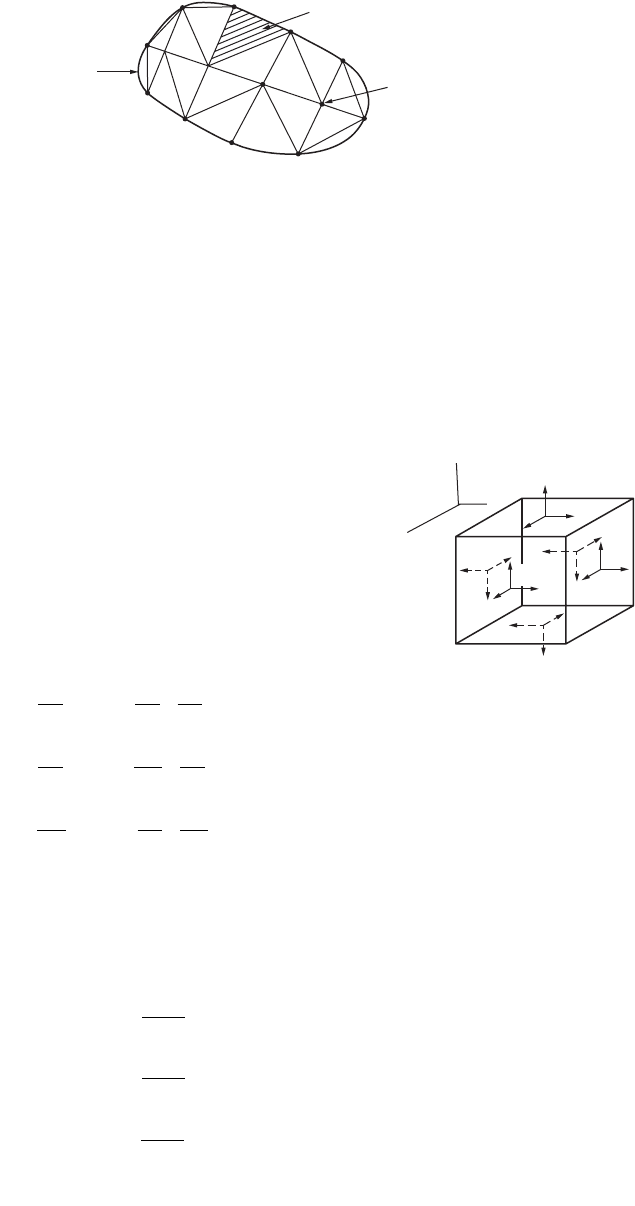
Figure 47.83 shows the state of stress in an elemental volume of a

body under load. It is deﬁned in terms of three normal stress com-

ponents s

x

, s

y

, and s

z

and three shear stress components t

xy

, t

yz

,

and t

zx

. The corresponding strain components are three normal

strains e

x

, e

y

, and e

z

and three shear strains g

xy

, g

yz

, and g

zx

. These

strain components are related to the displacement components u, v,

and w at a point as follows:

(47.149)

The relations given in Eq. (47.149) are valid in the case of the body experiencing small deformations. If

the body undergoes large or ﬁnite deformations, higher order terms must be retained.

The stress–strain equations for isotropic materials may be written in terms of Young’s modulus and

Poisson’s ratio as

(47.150)

FIGURE 47.82 Assemblage of subdivisions.

Boundary of

a region

Typical element

Typical node

FIGURE 47.83 State of stress in an

elemental volume.

x

z

y

0

τ

zy

σ

y

σ

z

τ

zx

τ

yx

τ

xz

τ

xy

τ

yz

τ

yz

τ

yx

σ

x

σ

y

P

x

xy

y

yz

z

zx

u

x

v

x

u

y

v

y

w

y

v

z

w

z

u

z

w

x

e

g

e

g

e

g

=

∂

=

∂

+

∂

=

∂

=

∂

+

∂

=

∂

=

∂

+

∂

x

2

xyz

y

2

yzx

z

2

zxy

xy

yz

zx

E

1

E

1

E

1

G, G , G

s

n

e

n

ee

s

n

e

n

ee

s

n

e

n

ee

t

g

t

g

t

g

=

-

++

()

[]

=

-

++

()

[]

=

-

++

()

[]

===

47-92 The Civil Engineering Handbook, Second Edition

Plane Stress

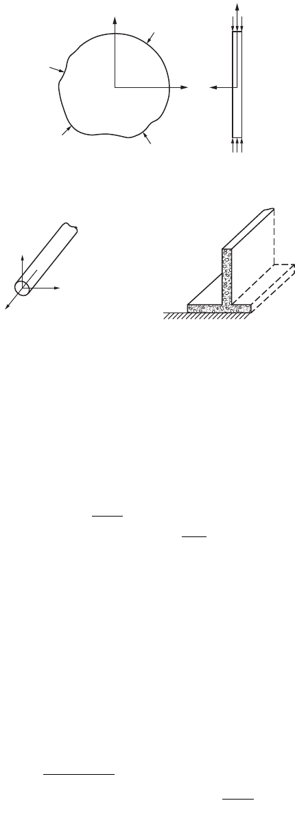
When the elastic body is very thin and there are no loads applied in the direction parallel to the thickness,

the state of stress in the body is said to be plane stress. A thin plate subjected to in-plane loading, as

shown in Fig. 47.84, is an example of a plane stress problem. In this case, s

z

= t

yz

= t

zx

= 0 and the

constitutive relation for an isotropic continuum is expressed as

(47.151)

Plane Strain

The state of plane strain occurs in members that are not free to expand in the direction perpendicular

to the plane of the applied loads. Examples of some plane strain problems are retaining walls, dams, long

cylinders, tunnels, etc., as shown in Fig. 47.85. In these problems e

z

, g

yz

, and g

zx

will vanish and hence

The constitutive relations for an isotropic material is written as

(47.152)

FIGURE 47.84 Plane stress problem.

FIGURE 47.85 Practical examples of plane strain problems.

y

x

z

y

x

y

z

s

n

e

g

x

y

xy

x

y

xy

E

È

Î

Í

˘

˚

˙

=

-

È

Î

Í

˘

˚

˙

È

Î

Í

˘

˚

˙

1

10

00

1

2

zxy

s

n

ss

=+

()

s

t

nn

n

e

g

x

y

xy

x

y

xy

E

È

Î

Í

˘

˚

˙

=

+

()

-

()

-

()

-

()

-

È

Î

Í

˘

˚

˙

È

Î

Í

˘

˚

˙

112

10

00

12

2

Theory and Analysis of Structures 47-93

Choice of Element Shapes and Sizes

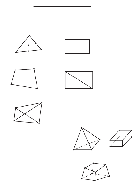
A ﬁnite element generally has a simple one-, two-, or three-dimensional conﬁguration. The boundaries

of elements are often straight lines, and the elements can be one-, two-, or three-dimensional, as shown

in Fig. 47.86. While subdividing the continuum, one has to decide the number, shape, size, and conﬁg-

uration of the elements in such a way that the original body is simulated as closely as possible. Nodes

must be located in locations where abrupt changes in geometry, loading, and material properties occur.

A node must be placed at the point of application of a concentrated load because all loads are converted

into equivalent nodal-point loads.

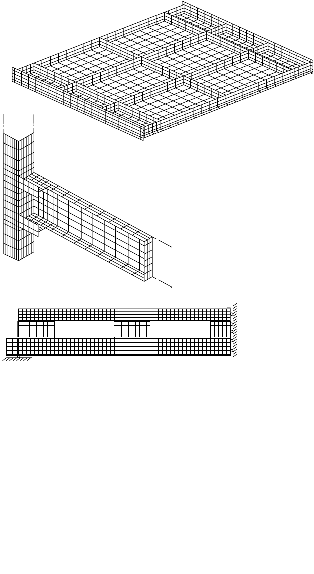
It is easy to subdivide a continuum into a completely regular one having the same shape and size. But

problems encountered in practice do not involve regular shape; they may have regions of steep gradients

of stresses. A ﬁner subdivision may be necessary in regions where stress concentrations are expected in

order to obtain a useful approximate solution. Typical examples of mesh selection are shown in Fig. 47.87.

Choice of Displacement Function

Selection of displacement function is the important step in the ﬁnite element analysis, since it determines

the performance of the element in the analysis. Attention must be paid to select a displacement function

that:

FIGURE 47.86 (a) One-dimensional element. (b) Two-dimensional element. (c) Three-dimensional element.

NODE 1 NODE 2

NODE 3

(a) One-dimensional Element

1

2

3

4

5

6

7

1

2

3

4

1

2

3

4

1

2

3

4

5

(b) Two-dimensional Element

1

2

3

4

12

3

4

5

6

7

8

1

2

3

4

5

6

7

8

(c) Three-dimensional Element

47-94 The Civil Engineering Handbook, Second Edition

1. has the number of unknown constants as the total number of degrees of freedom of the element.

2. does not have any preferred directions.

3. allows the element to undergo rigid-body movement without any internal strain.

4. is able to represent states of constant stress or strain.

5. satisﬁes the compatibility of displacements along the boundaries with adjacent elements.

Elements that meet both 3 and 4 are known as complete elements.

A polynomial is the most common form of displacement function. Mathematics of polynomials are

easy to handle in formulating the desired equations for various elements and convenient in digital

computation. The degree of approximation is governed by the stage at which the function is truncated.

Solutions closer to exact solutions can be obtained by including a greater number of terms. The poly-

nomials are of the general form

(47.153)

The coefﬁcient a’s are known as generalized displacement amplitudes. The general polynomial form for

a two-dimensional problem can be given as

FIGURE 47.87 Typical examples of ﬁnite element mesh.

Q

wx a a x a x a x

n

()

=+ + +º

+12 3

2

1

Theory and Analysis of Structures 47-95

in which

(47.154)

These polynomials can be truncated at any desired degree to give constant, linear, quadratic, or higher

order functions. For example, a linear model in the case of a two-dimensional problem can be given as

(47.155)

A quadratic function is given by

(47.156)

Pascal’s triangle, shown below, can be used for the purpose of achieving isotropy, i.e., to avoid displace-

ment shapes that change with a change in the local coordinate system.

Nodal Degrees of Freedom

The deformation of the ﬁnite element is speciﬁed completely by the nodal displacement, rotations, and/or

strains, which are referred to as degrees of freedom. Convergence, geometric isotropy, and potential energy

function are the factors that determine the minimum number of degrees of freedom necessary for a given

element. Additional degrees of freedom beyond the minimum number may be included for any element

by adding secondary external nodes, and such elements with additional degrees of freedom are called

higher order elements. The elements with more additional degrees of freedom become more ﬂexible.

Isoparametric Elements

The scope of ﬁnite element analysis is also measured by the variety of element geometries that can be

constructed. Formulation of element stiffness equations requires the selection of displacement expressions

with as many parameters as there are node point displacements. In practice, for planar conditions, only

the four-sided (quadrilateral) element ﬁnds as wide an application as the triangular element. The simplest

form of quadrilateral, the rectangle, has four node points and involves two displacement components at

each point, for a total of eight degrees of freedom. In this case one would choose four-term expressions

for both u and v displacement ﬁelds. If the description of the element is expanded to include nodes at

the midpoints of the sides, an eight-term expression would be chosen for each displacement component.

The triangle and rectangle can approximate the curved boundaries only as a series of straight line

segments. A closer approximation can be achieved by means of isoparametric coordinates. These are

nondimensionalized curvilinear coordinates whose description is given by the same coefﬁcients as are

1Constant

xy Linear

x

2

xy y

2

Quadratic

x

3

x

2

yxy

2

y

3

Cubic

x

4

x

3

yx

2

y

2

xy

3

y

4

Quantic

x

5

x

4

yx

3

y

2

x

2

y

3

xy

4

y

5

Quintic

uxy a a x ay ax axy ay ay

vxy a a a y a x a xy a y a y

m

n

mm m m m m m

n

,

()

=+ + + + + +º

()

=++ + + + +º+

++ + + + +

12 3 4

2

56

2

123 4

2

56

2

mi

i=1

n+1

=

Â

ua axay

va axay

=+ +

12 3

45 6

ua axayax axy ay

va axay a x a xy a y

=+ + + + +

= +++ + +

12 3 4

2

56

2

78 9 10

2

11 12

2

47-96 The Civil Engineering Handbook, Second Edition

employed in the displacement expressions. The displacement expressions are chosen to ensure continuity

across element interfaces and along supported boundaries, so that geometric continuity is ensured when

the same forms of expressions are used as the basis of description of the element boundaries. The elements

in which the geometry and displacements are described in terms of the same parameters and are of the

same order are called isoparametric elements. The isoparametric concept enables one to formulate ele-

ments of any order that satisfy the completeness and compatibility requirements and that have isotropic

displacement functions.

Isoparametric Families of Elements

Deﬁnitions and Justiﬁcations

For example, let u

i

represent nodal displacements and x

i

represent nodal x coordinates. The interpolation

formulas are

where N

i

and N are shape functions written in terms of the intrinsic coordinates. The value of u and the

value of x at a point within the element are obtained in terms of nodal values of u

i

and x

i

from the above

equations when the (intrinsic) coordinates of the internal point are given. Displacement components v

and w in the y and z directions are treated in a similar manner.

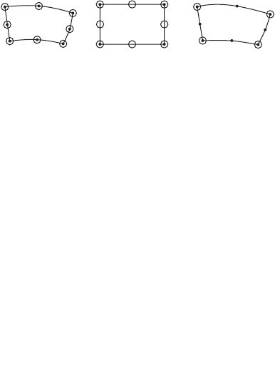
The element is isoparametric if m = n, N

i

= N, and the same nodal points are used to deﬁne both

element geometry and element displacement (Fig. 47.88a); the element is subparametric if m > n, the

order of N

i

is larger than N¢

i

(Fig. 47.88b); the element is superparametric if m < n, the order of N

i

is

smaller than N¢

i

(Fig. 47.88c). The isoparametric elements can correctly display rigid-body and constant-

strain modes.

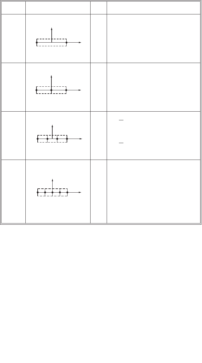
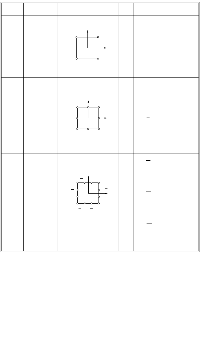
Element Shape Functions

The ﬁnite element method is not restricted to the use of linear elements. Most ﬁnite element codes

commercially available allow the user to select between elements with linear or quadratic interpolation

functions. In the case of quadratic elements, fewer elements are needed to obtain the same degree of

accuracy in the nodal values. Also, the two-dimensional quadratic elements can be shaped to model a

curved boundary. Shape functions can be developed based on the following properties:

1. Each shape function has a value of 1 at its own node and is zero at each of the other nodes.

2. The shape functions for two-dimensional elements are zero along each side that the node does

not touch.

3. Each shape function is a polynomial of the same degree as the interpolation equation. Shape

functions for typical elements are given in Fig. 47.89a and b.

Formulation of Stiffness Matrix

It is possible to obtain all the strains and stresses within the element and to formulate the stiffness matrix

and a consistent load matrix once the displacement function has been determined. This consistent load

matrix represents the equivalent nodal forces that replace the action of external distributed loads.

FIGURE 47.88 (a) Isoparametric element. (b) Subparametric element. (c) Superparametric element.

(a) (b) (c)

u x

i=1

m

i=1

n

==

¢

ÂÂ

Nu N x

ii i i

Theory and Analysis of Structures 47-97

As an example, let us consider a linearly elastic element of any of the types shown in Fig. 47.90. The

displacement function may be written in the form

(47.157)

in which {f} may have two components {u, v} or simply be equal to w, [P] is a function of x and y only,

and {A} is the vector of undetermined constants. If Eq. (47.157) is applied repeatedly to the nodes of the

element one after the other, we obtain a set of equations of the form

(47.158)

in which {D

*

} is the nodal parameters and [C] is the relevant nodal coordinates. The undetermined

constants {A} can be expressed in terms of the nodal parameters {D

*

} as

(47.159)

FIGURE 47.89 Shape functions for typical elements.

Five-node

quartic

element

Four-

node

cubic

element

Three-

node

parabolic

element

Two-node

linear

element

Element

name

Configuration DOF Shape functions

234

23

1

(−1,0)

1

(−1,0)

5

(1,0)

4

(1,0)

ξ

η

ξ

η

123

ξ

η

(−1,0)

(1,0)

12

ξ

η

+

N

i

=

1

−

2

(1

+

ξ

0

);

i

=

1, 2

N

i

=

1

−

2

ξ

0

(1

+

ξ

0

); i

=

1, 3

N

i

=

(1

−

ξ

2

); i

=

2

N

i

=

1

6

(1

+

ξ

0

)(9ξ

2

−

1)

i

=

1, 4

N

i

=

1

9

6

(1

+

9ξ

0

)(1

−

ξ

2

)

i

=

2, 3

N

i

=

1

−

6

(1

+

ξ

0

) {4ξ

0

(1

−

ξ

2

)

+

3ξ

0

}

i

=

1, 5

N

i

=

4ξ

0

(1

−

ξ

2

)(1

+

4ξ

0

)

i

=

2, 4

N

3

=

(1

−

4ξ

2

)(1

−

ξ

2

)

fPA

{}

=

[]

{}

DCA*

{}

=

[]

{}

ACD

{}

=

[]

{}

-1

*

47-98 The Civil Engineering Handbook, Second Edition

Substituting Eq. (47.159) into (47.157)

(47.160)

Constructing the displacement function directly in terms of the nodal parameters, one obtains

(47.161)

where [L] is a function of both (x, y) and (x, y)

i,j,m

given by

(47.162)

FIGURE 47.89 (continued).

Element

name

Configuration

η

ξ

(1,1)

(1,0)

(0,1)

(1,−1)

(−1,1)

(−1,0)

(−1,−1)

(0,−1)

4

1

2

3

4

6

7

5

8

3

1

23

4

5

6

7

8

10

9

11

12

(−

1

3

,1)

(

1

3

,1

)

(1,

1

3

)

(−1,

1

3

)

(

−1,−

1

3

)

(

1

3

,−1

)

(

−

1

3

,−1)

(

1,−

1

3

)

(1,1)

(1,−1)

(−1,−1)

(−1,1)

Four-node

plane

quadrilateral

Eight-node

plane

quadrilateral

Twelve-node

plane

quadrilateral

DOF

u, v

Shape functions

N

i

=

1

4

(1 + ξ

0

)(1 + η

0

);

N

i

=

1

4

(1 + ξ

0

)(1 + η

0

)

N

i

=

3

1

2

(1 + ξ

0

)(1 + η

0

)

N

i

=

3

9

2

(1 + ξ

0

)(1 + η

2

)

N

i

=

3

9

2

(1 + η

0

)(1 − ξ

2

)

N

i

=

1

2

(1 − ξ

2

)(1 + η

0

)

N

i

=

1

2

(1 − η

2

)(1 + ξ

0

)

i = 1, 2, 3, 4

i = 1, 3, 5, 7

i = 2,6

i = 4, 8

i = 1, 4, 7, 10

(ξ

0

+ η

0

− 1);

(−10 + 9(ξ

2

+ η

2

))

(1 + 9η

0

)

i = 5, 6, 11, 12

(1 + 9ξ

0

)

i = 2, 3, 8, 9

Serial

no.

1

2

3

fPCD

{}

=

[][]

{}

-1

*

fLD

{}

=

[]

{}

*

LPC

[]

=

[][]

-1

Theory and Analysis of Structures 47-99

The various components of strain can be obtained by appropriate differentiation of the displacement

function. Thus,

(47.163)

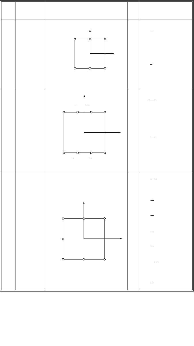
FIGURE 47.89 (continued).

(1,−1)

(−1,1)

(−1,−1)

(−1,−1) (1,−1)

(0,−1)

12

87

6

5

3

4

η

ξ

(0,1)

(1,1)

1

23

4

5

6

(−1,1)

(−1,0)

(−1,−1)

(1,−1)

(0,1)

(0,−1)

η

ξ

(1,1)

2

1

7

5

4

3

6

Serial

no.

Element

name

Configuration DOF Shape functions

4

Six-node

linear

quadrilateral

5

Eight-node

plane

quadrilateral

6

Seven-node

plane

quadrilateral

u, v

i = 1, 3, 4, 6

i = 2, 5

N

i

=

ξ

4

0

(1 + ξ

0

)(1 + η

0

)

N

i

=

1

2

(1 − ξ

2

)(1 + η

0

)

(1+η

0

)

(1+ η

0

)

i = 1, 4, 5, 8

i = 2, 3, 6, 7

N

i

=

3

9

2

(1 − ξ

2

)(1+9ξ

0

)

N

i

=

3

1

2

(1 + ξ

0

)( −1 + 9ξ

2

)

(1+ξ +η)

(1 + ξ − η)

N

5

=

1

2

(1 + η)(1 − ξ

2

)

N

6

= −

1

4

(1 − ξ)(1 + η)

N

7

=

1

2

(1 − ξ)(1 − η

2

)

N

3

=

ξ

4

(1 + ξ)(1 − η)

N

2

=

1

2

(1 − η)(1 − ξ

2

)

N

1

=

1

4

(1−ξ)(1 − η)

N

4

=

ξ

4

(1 + ξ)(1 + η)

(−

1

3

,1)

(−

1

3

,−1) (

1

3

,−1)

(

1

3

,1)

e

{}

=

[]

{}

BD*

47-100 The Civil Engineering Handbook, Second Edition

[B] is derived by differentiating appropriately the elements of [L] with respect to x and y. The stresses {s}

in a linearly elastic element are given by the product of the strain and a symmetrical elasticity matrix [E].

Thus,

or

(47.164)

The stiffness and the consistent load matrices of an element can be obtained using the principle of

minimum total potential energy. The potential energy of the external load in the deformed conﬁguration

of the element is written as

(47.165)

In Eq. (47.165) {Q

*

} represents concentrated loads at nodes, and {q} the distributed loads per unit

area. Substituting for {f}

T

from Eq. (47.161), one obtains

(47.166)

Note that the integral is taken over the area a of the element. The strain energy of the element integrated

over the entire volume v, is given as

Substituting for {e} and {s} from Eqs. (47.163) and (47.164), respectively,

(47.167)

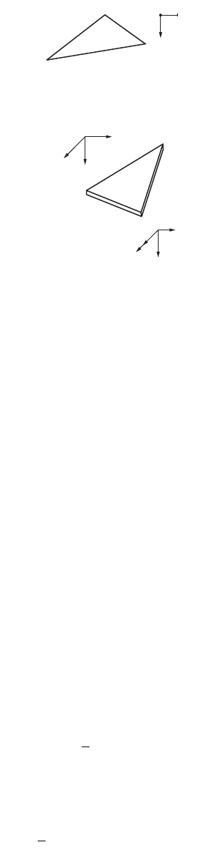
FIGURE 47.90 Degrees of freedom: (a) triangular plane stress element, (b) triangular bending element.

w

m

i

j

x

z

y

i

j

z

y

m

(a)

6 degrees

of freedom

(b)

θ

y

se

{}

=

[]

{}

E

s

{}

=

[][]

{}

EBD*

WDQ fqda

TT

a

=-

{}{}

-

{} {}

Ú

**

WDQ D Lqda

TTT

a

=-

{}{}

-

{}

[]

{}

Ú

** *

Udv

T

v

=

{} {}

Ú

1

2

es

UD BEBdvD

TT

v

=

{}

[][][]

Ê

Ë

Á

ˆ

¯

˜

{}

Ú

1

2

**

Wai-Fah Chen.The Civil Engineering Handbook

Подождите немного. Документ загружается.