Wai-Fah Chen.The Civil Engineering Handbook

Подождите немного. Документ загружается.

Theory and Analysis of Structures 47-161

Buckling of Shells

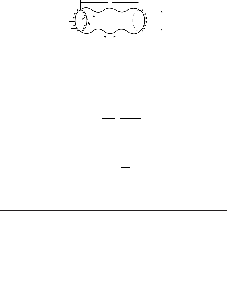
If a circular cylindrical shell is uniformly compressed in the axial direction, buckling symmetrical with

respect to the axis of the cylinder (Fig. 47.129) may occur at a certain value of the compressive load. The

critical value of the compressive force N

per unit length of the edge of the shell can be obtained by

solving the differential equation

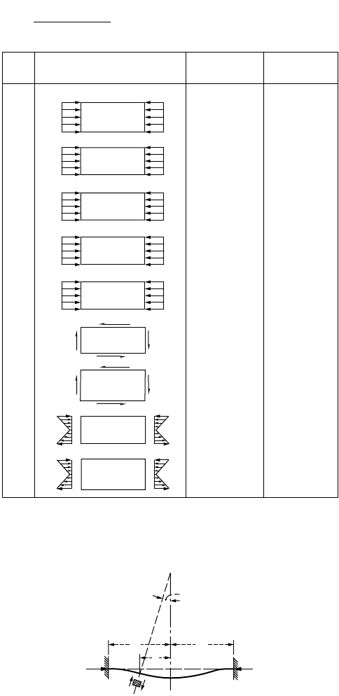
FIGURE 47.127 Values of K for plate with different boundary and loading conditions.

FIGURE 47.128 Circular plate under compressive loading.

s.s.

s.s. s.s.

s.s.

Fixed

s.s.

s.s. s.s.

Free

s.s. s.s.

Free

Fixed

s.s. s.s.

s.s.

Fixed

Fixed Fixed

Fixed

Fixed Fixed

Fixed

Case

Boundary condition

Type of

stress

(a)

(b)

(c)

(d)

(e)

(f)

(g)

(h)

(i)

Compression

Shear

Bending

Value of k for

long plate

4.0

6.97

0.425

1.277

5.34

8.98

23.9

41.8

5.42

12(1 − m

)(

)

47-162 The Civil Engineering Handbook, Second Edition

(47.357)

in which a is the radius of the cylinder and h is the wall thickness.

Alternatively, the critical force per unit length may also be obtained by using the energy method. For

a cylinder of length L, simply supported at both ends, one obtains

(47.358)

For each value of m there is a unique buckling mode shape and a unique buckling load. The lowest value

is of greatest interest and is thus found by setting the derivative of N

with respect to L equal to zero for

m = 1. With Poisson’s ratio equal to 0.3, the buckling load is obtained as

(47.359)

It is possible for a cylindrical shell to be subjected to uniform external pressure or to the combined action

of axial and uniform lateral pressure.

47.13 Dynamic Analysis

Equation of Motion

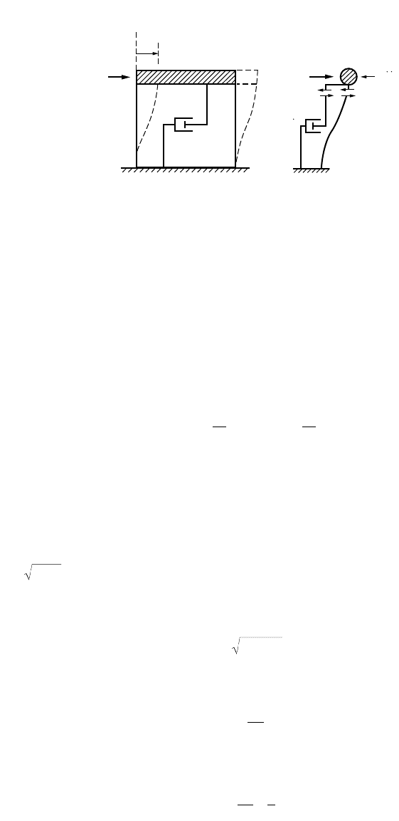
The essential physical properties of a linearly elastic structural system subjected to external dynamic

loading are its mass, stiffness properties, and energy absorption capability or damping. The principle of

dynamic analysis may be illustrated by considering a simple single-story structure, as shown in Fig. 47.130.

The structure is subjected to a time-varying force f(t). k is the spring constant that relates the lateral

story deﬂection x to the story shear force, and the dash pot relates the damping force to the velocity by

a damping coefﬁcient c. If the mass, m, is assumed to concentrate at the beam, the structure becomes a

single-degree-of-freedom (SDOF) system. The equation of motion of the system may be written as

(47.360)

Various solutions to Eq. (47.360) can give insight into the behavior of the structure under dynamic

situations.

Free Vibration

In this case the system is set to motion and allowed to vibrate in the absence of applied force f(t). Letting

f(t) = 0, Eq. (47.360) becomes

FIGURE 47.129 Buckling of a cylindrical shell.

0++=

EhL

Da m

222

= 0 605

mx cx kx f t

˙˙ ˙

++ =

()

Theory and Analysis of Structures 47-163

(47.361)

Dividing Eq. (47.361) by the mass, m, we have

(47.362)

where

(47.363)

The solution to Eq. (47.362) depends on whether the vibration is damped or undamped.

Example 47.16: Undamped Free Vibration

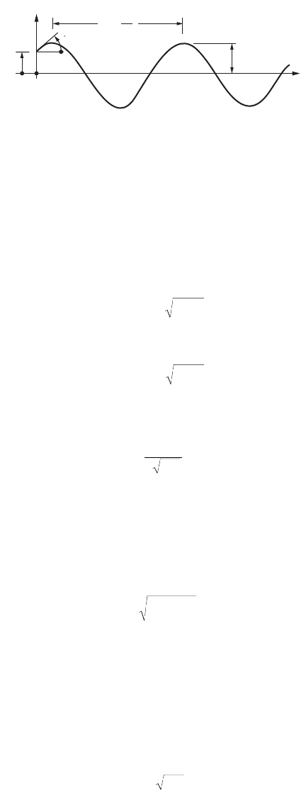
In this case, c = 0, and the solution to the equation of motion may be written as

(47.364)

where is the circular frequency. A and B are constants that can be determined by the initial

boundary conditions. In the absence of external forces and damping, the system will vibrate indeﬁnitely

in a repeated cycle of vibration with an amplitude of

(47.365)

and a natural frequency of

(47.366)

The corresponding natural period is

(47.367)

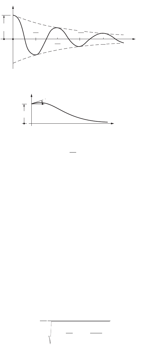
The undamped free vibration motion, as described by Eq. (47.364), is shown in Fig. 47.131.

FIGURE 47.130 (a) One DOF structure. (b) Forces applied to structures.

f(t)

(a) 1 DOF Structure

(b) Forces applied

to structure

f(t)

mx cx kx

˙˙ ˙

++ =0

˙˙ ˙

xxx++=20

xw w

2xw w==

and

xA tB t=+sin cosww

w= km/

XAB=+

f =

21p

47-164 The Civil Engineering Handbook, Second Edition

Example 47.17: Damped Free Vibration

If the system is not subjected to applied force and damping is presented, the corresponding solution

becomes

(47.368)

where

(47.369)

and

(47.370)

The solution of Eq. (47.368) changes its form with the value of x, deﬁned as

(47.371)

If x

< 1, the equation of motion becomes

(47.372)

where x

is the damped angular frequency deﬁned as

(47.373)

For most building structures x is very small (about 0.01), and therefore w

ª w. The system oscillates

about the neutral position as the amplitude decays with time t. Figure 47.132 illustrates an example of

such motion. The rate of decay is governed by the amount of damping present.

If the damping is large, then oscillation will be prevented. This happens when x

> 1; the behavior is

referred to as overdamped. The motion of such behavior is shown in Fig. 47.133.

Damping with x

= 1 is called critical damping. This is the case where minimum damping is required

to prevent oscillation, and the critical damping coefﬁcient is given as

(47.374)

where k and m are the stiffness and mass of the system, respectively.

The degree of damping in the structure is often expressed as a proportion of the critical damping

value. Referring to Eqs. (47.371) and (47.375), we have

FIGURE 47.131 Response of undamped free vibration.

x(t)

x(0)

2π

T =

x(0)

xA t B t=

()

exp expll

lwx x

1=-+ -

[]

lwxx

1=-- -

[]

mk2

xtAtBt

()

exp cos sinxw w w

wxw

()

ckm

= 2

Theory and Analysis of Structures 47-165

(47.375)

x is called the critical damping ratio.

Forced Vibration

If a structure is subjected to a sinusoidal motion such as a ground acceleration of , it will

oscillate, and after some time the motion of the structure will reach a steady state. For example, the

equation of motion due to the ground acceleration (from Eq. (47.362)) is

(47.376)

The solution to the above equation consists of two parts: the complimentary solution given by Eq. (47.364)

and the particular solution. If the system is damped, oscillation corresponding to the complementary

solution will decay with time. After some time the motion will reach a steady state, and the system will

vibrate at a constant amplitude and frequency. This motion, which is called force vibration, is described

by the particular solution expressed as

(47.377)

It can be observed that the steady force vibration occurs at the frequency of the excited force, w

, not at

the natural frequency of the structure, w.

Substituting Eq. (47.377) into (47.376), the displacement amplitude can be shown to be

(47.378)

FIGURE 47.132 Response of damped free vibration.

FIGURE 47.133 Response of free vibration with critical damping.

x(t)

x(0)

2π

4π

3π

x(t)

x(0)

˙˙

sinxF t

˙˙ ˙

sinxxxFt

++=-2

xw w w

xC tC t

sin cosww

47-166 The Civil Engineering Handbook, Second Edition

The term –F/w

is the static displacement caused by the force due to the inertia force. The ratio of the

response amplitude relative to the static displacement –F/w

is called the dynamic displacement ampli-

ﬁcation factor, D, given as

(47.379)

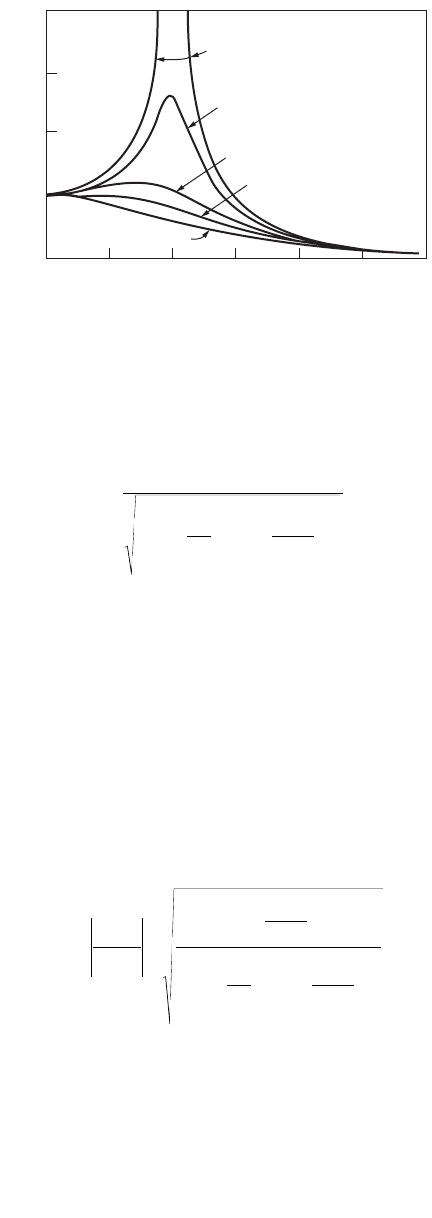
The variation of the magniﬁcation factor with the frequency ratio w

/w and damping ratio x is shown

in Fig. 47.134.

When the dynamic force is applied at a frequency much lower than the natural frequency of the system

/w  1), the response is quasistatic. The response is proportional to the stiffness of the structure, and

the displacement amplitude is close to the static deﬂection.

When the force is applied at a frequency much higher than the natural frequency (w

/w  1), the

response is proportional to the mass of the structure. The displacement amplitude is less than the static

deﬂection (D < 1).

When the force is applied at a frequency close to the natural frequency, the displacement amplitude

increases signiﬁcantly. The condition at which w

/w = 1 is known as resonance.

Similarly, the ratio of the acceleration response relative to the ground acceleration may be expressed as

(47.380)

is called the dynamic acceleration magniﬁcation factor.

Response to Suddenly Applied Load

Consider the spring–mass damper system of which a load P

is applied suddenly. The differential equation

is given by

(47.381)

FIGURE 47.134 Vibration of dynamic ampliﬁcation factor with frequency ratio.

012

/ω

ξ = 0

ξ = 0.2

ξ = 0.5

ξ = 0.7

ξ = 1.0

˙˙ ˙˙

˙˙

Mx cx kx P

˙˙ ˙

++ =

Theory and Analysis of Structures 47-167

If the system is started at rest, the equation of motion is

(47.382)

If the system is undamped, then x = 0 and w

= w; we have

(47.383)

The maximum displacement is 2(P

/k), corresponding to cos w

t = –1. Since P

/k is the maximum static

displacement, the dynamic ampliﬁcation factor is 2. The presence of damping would naturally reduce

the dynamic ampliﬁcation factor and the force in the system.

Response to Time-Varying Loads

Some forces and ground motions that are encountered in practice are rather complex in nature. In

general, numerical analysis is required to predict the response of such effects, and the ﬁnite element

method is one of the most common techniques to be employed in solving such problems.

The evaluation of responses due to time-varying loads can be carried out using the piecewise exact

method. In using this method, the loading history is divided into small time intervals. Between these

points, it is assumed that the slope of the load curve remains constant. The entire load history is

represented by a piecewise linear curve, and the error of this approach can be minimized by reducing

the length of the time steps. A description of this procedure is given in Clough and Penzien (1993).

Other techniques employed include Fourier analysis of the forcing function, followed by solution for

Fourier components in the frequency domain. For random forces, the random vibration theory and

spectrum analysis may be used (Dowrick, 1988; Warburton, 1976).

Multiple Degree Systems

In multiple degree systems, an independent differential equation of motion can be written for each degree

of freedom. The nodal equations of a multiple degree system consisting of n degrees of freedom may be

written as

(47.384)

where [m] = a symmetrical n x n matrix of mass

[c] = a symmetrical n x n matrix of damping coefﬁcient

{F(t)} = the force vector, which is zero in the case of free vibration

Consider a system under free vibration without damping; the general solution of Eq. (47.384) is

assumed in the form of

(47.385)

where angular frequency w and phase angle f are common to all x’s. In this assumed solution, f and C

, … C

are the constants to be determined from the initial boundary conditions of the motion, and

w is a characteristic value (eigenvalue) of the system.

tt t

=--

()

1 exp cos sinxw w

[]

1 cosw

mx cx kx Ft

[]

{}

[]

{}

[]

{}

()

{}

˙˙ ˙

n n

000

MMMM

()

cos

47-168 The Civil Engineering Handbook, Second Edition

Substituting Eq. (47.385) into Eq. (47.384) yields

(47.386)

(47.387)

where [k] and [m] are the n ¥ n matrices, w

and cos(wt – f) are scalars, and {C} is the amplitude vector.

For nontrivial solution, cos(wt – f) π 0; thus solution to Eq. (47.387) requires the determinant of [[k] –

[m]] = 0. The expansion of the determinant yields a polynomial of n degree as a function of w

, the

n roots of which are the eigenvalues w

, w

, … w

If the eigenvalue w for a normal mode is substituted in Eq. (47.387), the amplitude vector {C} for that

mode can be obtained. {C

}, {C

}, … {C

} are therefore called eigenvectors, the absolute values that

must be determined through initial boundary conditions. The resulting motion is a sum of n harmonic

motions, each governed by the respective natural frequency w, written as

(47.388)

Distributed Mass Systems

Although many structures may be approximated by lumped mass systems, in practice all structures are

distributed mass systems consisting of an inﬁnite number of particles. Consequently, if the motion is

repetitive, the structure has an inﬁnite number of natural frequency and mode shapes. The analysis of a

distributed-parameter system is entirely equivalent to that of a discrete system once the mode shapes

and frequencies have been determined, because in both cases the amplitudes of the modal response

components are used as generalized coordinates in deﬁning the response of the structure.

In principle an inﬁnite number of these coordinates are available for a distributed-parameter system,

but in practice only a few modes, usually those of lower frequencies, will provide signiﬁcant contribute

to the overall response. Thus the problem of a distributed-parameter system can be converted to a discrete

system form in which only a limited number of modal coordinates is used to describe the response.

Flexural Vibration of Beams

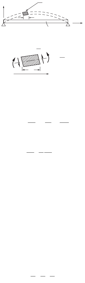
The motion of the distributed mass system is best illustrated by a classical example of a uniform beam

with of span length L, a ﬂexural rigidity EI, and a self-weight of m per unit length, as shown in Fig. 47.135a.

The beam is free to vibrate under its self-weight. From Fig. 47.135b, dynamic equilibrium of a small

beam segment of length dx requires:

(47.389)

in which

(47.390)

km km km

km km k m

km km km

nn n n nn nn

11 11

12 12

21 21

22 22

-- -

ww w

M MMM

cos --

()

kmC

[]

{}

xC t

{}

()

cos

∂

dx mdx

∂

Theory and Analysis of Structures 47-169

and

(47.391)

Substituting these equations into Eq. (47.389) leads to the equation of motion of the ﬂexural beam:

(47.392)

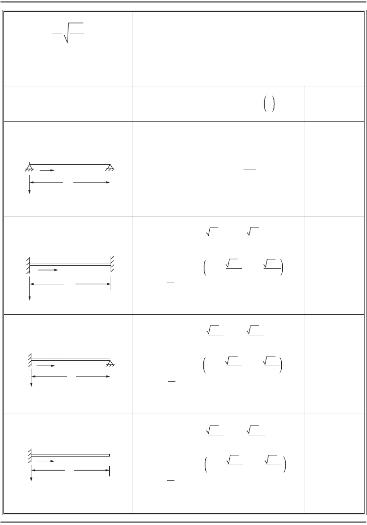
Equation (47.392) can be solved for beams with given sets of boundary conditions. The solution consists

of a family of vibration modes with corresponding natural frequencies. Standard results are available in

Table 47.5 to compute the natural frequencies of uniform ﬂexural beams of different supporting condi-

tions. Methods are also available for dynamic analysis of continuous beams (Clough and Penzien, 1993).

Shear Vibration of Beams

Beams can deform by ﬂexure or shear. Flexural deformation normally dominates the deformation of

slender beams. Shear deformation is important for short beams or in higher modes of slender beams.

Table 47.6 gives the natural frequencies of uniform beams in shear, neglecting ﬂexural deformation. The

natural frequencies of these beams are inversely proportional to the beam length L rather than L

, and

the frequencies increase linearly with the mode number.

Combined Shear and Flexure

The transverse deformation of real beams is the sum of ﬂexure and shear deformations. In general,

numerical solutions are required to incorporate both the shear and ﬂexural deformation in the prediction

of the natural frequency of beams. For beams with comparable shear and ﬂexural deformations, the

following simpliﬁed formula may be used to estimate the beam’s frequency:

(47.393)

where f is the fundamental frequency of the beam and f

and f

are the fundamental frequencies predicted

by the ﬂexure and shear beam theories, respectively (Rutenberg, 1975).

FIGURE 47.135 (a) Beam in ﬂexural vibration. (b) Equilibrium of beam segment in vibration.

Small element

beam

(a)

(b)

∂V

∂x

V +

∂M

∂x

M +

=- =-

∂

111

222

fff

47-170 The Civil Engineering Handbook, Second Edition

Natural Frequency of Multistory Building Frames

Ta ll building frames often deform more in the shear mode than in ﬂexure. The fundamental frequencies

of many multistory building frameworks can be approximated by (Housner and Brody, 1963; Rinne, 1952)

TA BLE 47.5 Frequencies and Mode Shapes of Beams in Flexural Vibration

Fixed - Fixed

Pinned - Pinned

Fixed - Pinned

Cantilever

Boundary conditions

n = 1, 2, 3...

L = Length (m)

EI = Flexural rigidity (Nm

)

M = Mass per unit length (kg/m)

;

n = 1,2,3

Mode shape y

−

;

n = 1,2,3...

(nπ)

nπx

sin

cosh

− cos

− A

sin h

− sin

cosh

− cos

− A

sin h

− sin

cosh

− cos

− A

sin h

− sin

(2n−1)

;

n > 5

0.73410

1.01847

0.99922

1.00003

1.0; n > 4

3.52

22.03

61.69

120.90

199.86

(4n + 1)

;

n > 5

15.42

49.96

104.25

178.27

272.03

1.0; n > 3

1.00078

1.00000

n > 5

(2n + 1)

;

22.37

61.67

120.90

199.86

298.55

1.0; n > 5

0.98250

1.00078

0.99997

1.00000

0.99999