Wai-Fah Chen.The Civil Engineering Handbook

53-22 The Civil Engineering Handbook, Second Edition

where

(53.97)

Equation (53.96) is called the characteristic equation of A, or the eigenvalue equation. The matrix (A – lI)

is called the characteristic matrix. There are n roots for Eq. (53.96), counting multiplicity. These are the

n eigenvalues of A, l

1

, l

2

, …, l

n

. For an eigenvalue l

i

, we solve the set of (homogeneous) linear equations

(A – l

i

I)x = 0 to determine the components of the corresponding eigenvector x

i

. In general, l

i

and x

i

are either real or complex numbers and vectors, respectively.

If the matrix A is symmetric, then:

1. The eigenvalues are real.

2. The eigenvectors are all mutually orthogonal; that is,

Bilinear and Quadratic Forms

If A is a square matrix of order n and x and y are two arbitrary n vectors, then the scalar

(53.98)

is called a bilinear form. If, however, the matrix A is also symmetric, then

(53.99)

is called a quadratic form with the kernel A.

The matrix A is called positive deﬁnite if v > 0 for all x π 0, and we write A > 0. If v ≥ 0 for all x and

there exists a nonzero vector x for which equality holds, we say A is positive semideﬁnite (or nonnegative

deﬁnite) and write A ≥ 0. There are corresponding deﬁnitions for negative deﬁnite (or nonpositive deﬁnite).

If there exist vectors x

1

and x

2

such that x

T

1

Ax

1

> 0 and x

T

2

Ax

2

< 0, we say A is indeﬁnite.

For a positive deﬁnite matrix A it is necessary and sufﬁcient that

A quadratic form represents, in general, a conic section of some kind. Considering the two-dimen-

sional case for simplicity, we write

(53.100)

or

which is the equation of an ellipse.

b

n

1=

b

n 1–

a

11

a

22

L a

nn

+++ a

ii

i 1=

n

Â

tr A() trace of A====

M

b

nr–

sum of all principal minors of order r of A=

M

b

0

A determinant of A==

x

i

T

x

j

x

j

T

x

i

0==

u x

T

Ay=

v x

T

Ax=

a

11

0

a

11

a

12

a

21

a

22

0 L A 0>,,>,>

x

T

Ax b with A symmetric=

a

11

x

1

2

2a

12

x

1

x

2

a

22

x

2

++b=

General Mathematical and Physical Concepts 53-23

53.6 Coordinate Transformations

Linear Transformations

A general linear transformation of a vector x to another vector y takes the form

(53.101)

Each element of the y vector is a linear combination of the elements of x plus a translation or shift

represented by an element of the t vector. The matrix M is called the transformation matrix, which is in

general rectangular, and t is called the translation vector. For our use we restrict M to being square

nonsingular; thus, the inverse relation exists, or

(53.102)

in which case it is called afﬁne transformation. Although both Eqs. (53.101) and (53.102) apply to higher-

dimension vectors, we will limit our discussions, without loss of generality, to the more practical two-

and three-dimensional spaces, where the elements of the transformations can be depicted geometrically.

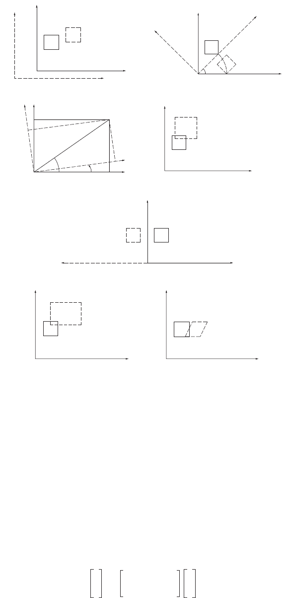
Two-Dimensional Linear Transformations

There are six elementary transformations, each representing a single effect, which are geometrically

represented in Fig. 53.3. Initially, four vectors (1,3) (1,5), (3,3) (3,5) representing the corners of a square

(solid lines in Fig. 53.3) are referred to the x

1

, x

2

coordinate system. Each of the six elementary transfor-

mations operates on the square, and the resulting y

1

, y

2

coordinates are plotted to show the effect on the

location, orientation, size, and shape of the square after the transformation (dashed lines in Fig. 53.3).

In displaying the effects of the transformations, we either display the new ﬁgure (dashed lines) in the

same coordinate system, or we change the coordinate system. It is easier for the student to visualize these

transformations if the new ﬁgure is drawn without changing the coordinate system, which we did in

Fig. 53.3. However, as we discuss each elementary transformation, we will comment on the second

interpretation when appropriate.

1. Translation

(53.103)

The square is shifted 3 units in x

1

direction and 1 unit in x

2

direction, as shown in Fig. 53.3(a).

Alternatively, the solid square remains and the coordinate axes shifted (in the opposite direction

and shown in dashed lines).

2. Uniform Scale

(53.104)

The (dotted) square is enlarged by the uniform scale u (= 1.5 in Fig. 53.3(b)), which results from

all four point coordinate pairs multiplied by u. Alternatively, the solid square is referred to the same

coordinate system, except that the units along the axes are now 1/u of the original units.

3. Rotation

(53.105)

yMxt+=

xM

1–

yt–()=

yxt where M+ I==

yMx M U

u 0

0 u

uI====

yMx MR

b

cos

b

sin

b

sin–

b

cos

===

53-24 The Civil Engineering Handbook, Second Edition

The square retains its shape, but is rotated through b about the origin of the coordinate system.

In Fig. 53.3(c), the coordinate system is also rotated (45˚). The elements of R are derived from

Fig. 53.3(d) as follows:

or

(53.106)

FIGURE 53.3 (a) Translation. (b) Uniform scale. (c) Rotation. (d) Rotation of a two-dimensional coordinate system.

(e) Reﬂection. (f) Stretch (nonuniform scale). (g) Skew (nonperpendicularity of axes).

(a) (c)

(d)

(e)

(f)

(g)

(b)

x

2

,

y

2

x

2

,

y

2

x

2

,

y

2

x

2

,

y

2

x

2

,

y

2

x

2

,

y

2

45°

y

2

x

2

x

1

P

y

1

y

2

x

2

y

1

x

1

r

0

Θ

b

x

1

,

y

1

x

1

,

y

1

x

1

,

y

1

x

1

,

y

1

x

1

,

y

1

x

1

,

y

1

y

1

r

qb

–()cos r

qb

r

qb

sinsin+coscos==

y

2

r

qb

–()sin r

qb

r–

qb

sincoscossin==

y

1

x

1

b

cos x

2

b

y

2

x

1

–

b

sin x

2

b

cos+=

sin+=

y

1

y

2

b

cos

b

sin

b

sin–

b

cos

x

1

x

2

=

General Mathematical and Physical Concepts 53-25

The matrix R is proper orthogonal, R

–1

= R

T

and |R| = +1. Rotation matrices do not change the

length of the vector, i.e., |x| = |y|. Considering the square of the vector length,

or

which for a nontrivial solution means that M

T

M = I, thus showing that M is an orthogonal matrix.

4. Reﬂection

Figure 53.3(e) shows reﬂection of the x

1

axis (i.e., about the x

2

axis). F is improper orthogonal,

F

–1

= F

T

= F and |F| = –1.

5. Stretch (Two Scale Factors)

(53.107)

The square is transformed into a rectangle as shown in Fig. 53.3(f), in which

6. Skew (Shear)

(53.108)

The square is transformed into a parallelogram as shown in Fig. 53.3(g), where

From these elementary transformations several afﬁne transformations may be constructed using var-

ious sequences. The following are two of the commonly used transformations in photogrammetry.

Four-Parameter Transformation.

(53.109a)

or

(53.109b)

y

T

yMx()

T

Mx x

T

M

T

Mx

T

x

T

x===

x

T

M

T

MI–()x 0=

yMx MF

1– 0

01

===

yMx MS

s

1

0

0 s

2

===

S

2 0

0 1.5

=

yMx MK

1 k

01

===

K

1 0.5

01

=

y

1

y

2

u 0

0 u

b

cos

b

sin

b

sin–

b

cos

x

1

x

2

t

1

t

2

+=

y

1

ux

1

b

ux

2

b

t

1

y

2

u– x

1

b

ux

2

b

t

2

+cos+sin=

+sin+cos=

53-26 The Civil Engineering Handbook, Second Edition

or

(53.109c)

or

(53.109d)

The inverse transformation is given by

(53.109e)

or

(53.109f)

This transformation has four parameters: a uniform scale, a rotation, and two translations. It is a

conformal transformation.

Six-Parameter Transformation.

(53.110a)

or

(53.110b)

The six parameters of this transformation consist of two scales, one skew factor (lack of perpendicularity

of the axes), one rotation, and two shifts. The inverse transformation is given by

(53.110c)

Three-Dimensional Linear Transformations

As in the two-dimensional case, afﬁne transformation in three dimensions can be factored out in several

elementary transformations: translation, uniform scale, nonuniform scale, rotations, reﬂections, etc.

Consideration, however, is limited to the seven-parameter transformation, which is composed of a

uniform scale change, three translations, and three rotations.

We ﬁrst consider rotations in three-dimensional space.

Rotations of a Three-Dimensional Coordinate System. There are three elementary rotations, one about

each of the three axes. They are frequently performed in sequence one after the other. A set of three of

these is as follows, where x is the original system, x¢ is once rotated, and x≤ is twice rotated:

y

1

ax

1

bx

2

c

y

2

b– x

1

ax

2

d++=

++=

y

1

y

2

a b

b – a

x

1

x

2

c

d

+=

x

1

x

2

1

u

---

b

cos

b

sin–

b

sin

b

cos

y

1

c–

y

2

d–

=

x

1

x

2

1

a

2

b

2

+

----------------

a b–

b a

y

1

c–

y

2

d–

=

y

1

y

2

s

1

0

0 s

2

1 k

0 1

b

cos

b

sin

b

sin–

b

cos

x

1

x

2

t

1

t

2

+=

y

1

y

2

a b

d e

x

1

x

2

c

f

+=

x

1

x

2

1

ae bd–

-----------------

e b–

d– a

y

1

c–

y

2

f–

=

General Mathematical and Physical Concepts 53-27

1. b

1

about x

1

axis, positive rotation advances +x

2

to +x

3

2. b

2

about x¢

2

axis, positive rotation advances +x¢

3

to +x¢

1

3. b

3

about x≤

3

axis, positive rotation advances +x≤

1

to +x≤

2

Each of the three elementary rotations is represented in matrix form by

(53.111a)

where x

1

, x

2

, x

3

are the coordinates before rotation and x¢

1

, x¢

2

, x ¢

3

are the coordinates after rotation.

Similarly, rotations of +b

2

about the x ¢

2

axis and +b

3

about the x≤

3

axis are given by

(53.111b)

(53.111c)

The three rotations in Eq. (53.111) are often referred to as elementary rotations, since they may be

used to construct any required set of sequential rotations. By successive substitution, the total rotation

matrix is obtained:

(53.112)

in which M is now a function of the three rotation angles b

1

, b

2

, b

3

. The most commonly used set of

sequential rotations (in photogrammetry) is given the symbols w, f, k where w ∫ b

1

; f ∫ b

2

; k ∫ b

3

. In this

case, the matrix M which rotates the object coordinate system (X, Y, Z) parallel to the photo coordinate

system (x, y, z) is given by

(53.113)

in which w is about the X axis, f is about the once-rotated Y axis, and k is about the twice-rotated Z

axis. The matrix M is orthogonal, since M

w

, M

f

, and M

k

are each orthogonal.

Seven-Parameter Transformation. This transformation contains seven parameters: a uniform scale

change u, three rotations b

1

, b

2

, b

3

, and three translations t

1

, t

2

, t

3

. It takes the general form

y = uMx + t (53.114)

The orthogonal matrix M is a function of only three independent parameters, in this case the angles

b

1

, b

2

, b

3

. This transformation is useful for different applications, such as absolute orientation, model

connection, etc.

The orthogonal matrix M may be constructed by other methods besides sequential rotations. Two

such methods follow.

x

1

¢

x

2

¢

x

3

¢

10 0

0

b

1

cos

b

1

sin

0

b

1

sin–

b

1

cos

x

1

x

2

x

3

M

b

1

x

1

x

2

x

3

==

x

1

≤

x

2

≤

x

3

≤

b

2

cos 0

b

2

sin–

0 1 0

b

2

sin 0

b

1

cos

x

1

¢

x

2

¢

x

3

¢

M

b

2

x

1

x

2

x

3

==

y

1

y

2

y

3

x

1

≤¢

x

2

≤¢

x

3

≤¢

b

3

cos

b

3

sin 0

b

3

sin–

b

3

cos 0

00 1

x

1

≤

x

2

≤

x

3

≤

M

b

3

x

1

≤

x

2

≤

x

3

≤

== =

yx

≤¢

M

b

3

M

b

2

M

b

1

xMx== =

M

fk

coscos

fk

sincos–

f

sin

wk

wfk

cossinsin+sincos

wk

wfk

sinsinsin–coscos

w

sin– fcos

w

sin

k

w

cos

fk

cossin–sin

w

sin

k

w

cos

fk

sinsin+cos

wf

coscos

=

53-28 The Civil Engineering Handbook, Second Edition

Constructing M by One Rotation about a Line. This is also often referred to as the solid body rotation.

Given a three-dimensional object in two different orientations, there exists a line in space about which

the object may be rotated by a ﬁnite angle to change it from one orientation to the other. If the said line

has l, m, n as direction cosines and the angle of rotation is designated by a, the rotation matrix is given by

(53.115)

A Purely Algebraic Derivation of M. The following skew-symmetric matrix contains only three param-

eters a, b, c:

(53.116a)

An orthogonal matrix M can be obtained from M using

(53.116b)

in which M is the identity matrix. Then

(53.117)

Nonlinear Transformations

In addition to the linear transformations discussed so far, we use nonlinear transformations both in two

and three dimensions. In two dimensions we have the following two transformations:

Eight-Parameter Transformation. The equations

(53.118a)

represent the projective transformation from the x to the y coordinate systems, with the eight transfor-

mation parameters being a

0

, b

0

, a

1

, …, c

2

. Its inverse is given by

(53.118b)

These equations describe the central projectivity between two planes.

M

l

2

1

a

cos–()

a

cos+

lm

1

a

cos–()

na

sin+

ln

1

a

cos–()

ma

sin–

lm

1

a

cos–()

na

sin–

m

2

1

a

cos–()

a

cos+

mn

1

a

cos–()l

a

sin+

ln

1

a

cos–()m

a

sin+

mn

1

a

cos–()

la

sin–

n

2

1

a

cos–()

a

cos+

=

S

0 c– b

c 0 a–

b– a 0

=

MIS+()IS–()

1–

IS–()

1–

IS+()==

MIS–()

1–

IS+()=

1

1 a

2

b

2

c

2

+++

-----------------------------------

1 a

2

b

2

– c

2

–+ 2ab 2c– 2ac 2b+

2ab 2c+ 1 a

2

– b

2

c

2

–+ 2bc 2a–

2ac 2b– 2bc 2a + 1 a

2

– b

2

– c

2

+

=

y

1

a

1

x

1

b

1

x

2

c

1

++

a

0

x

1

b

0

x

2

1++

------------------------------------=

y

2

a

2

x

1

b

2

x

2

c

2

++

a

0

x

1

b

0

x

2

1++

------------------------------------=

x

1

c

1

y

1

–()b

0

y

2

b

2

–()c

2

y

2

–()b

0

y

1

b

1

–()–

a

0

y

1

a

1

–()b

0

y

2

b

2

–()a

2

y

2

a

2

–()b

0

y

1

b

1

–()–

------------------------------------------------------------------------------------------------------------=

x

2

a

0

y

1

a

1

–()c

2

y

2

–()a

0

y

2

a

2

–()c

1

y

1

–()–

a

0

y

1

a

1

–()b

0

y

2

b

2

–()a

0

y

2

a

2

–()b

0

y

1

b

1

–()–

------------------------------------------------------------------------------------------------------------=

General Mathematical and Physical Concepts 53-29

Tw o-Dimensional General Polynomials.

(53.119a)

These polynomials can obviously be extended to higher powers in x

1

, x

2

. A special case of these is the

conformal form given in the following section.

Tw o-Dimensional Conformal Polynomials. The conformal property preserves the angles between inter-

secting lines after the transformation. If we impose the two conditions

(53.119b)

on the general polynomials in Eq. (53.119a), we get

(53.119c)

Note that the ﬁrst three terms after the equal signs are the same as those in the four-parameter

transformation given in Eq. (53.109c). Equation (53.119c) can also be derived using complex numbers

by writing

in which . Expanding and equating y

1

to the real part and y

2

to the imaginary part (multiplier

of i) on the right-hand side leads to Eq. (53.119c).

Three-dimensional General Polynomials.

(53.120a)

We can extend these polynomials to higher order. Unlike the two-dimensional case, conformal trans-

formation does not exist in three dimensions beyond the ﬁrst-order (or linear) case given by the seven-

parameter transformation, Eq. (53.114). A close approximation, which exists for only second-degree

terms, is derived by imposing conditions similar to those in Eq. (53.119b) on every pair of coordinates

in Eq. (53.120a). This makes the projections of the 3-space onto each of the three planes conformal.

Thus, imposing the following on the general polynomials in Eq. (53.120a)

(53.120b)

leads to

(53.120c)

y

1

a

0

a

1

x

1

a

2

x

2

a

3

x

1

x

2

a

4

x

1

2

a

5

x

2

L+++ +++=

y

2

b

0

b

1

x

1

b

2

x

2

b

3

x

1

x

2

b

4

x

1

2

b

5

x

2

L+++ +++=

∂

y

1

∂

x

1

--------

∂

y

2

∂

x

2

--------

and

∂

y

1

∂

x

2

--------

∂

y

2

∂

x

1

--------–==

y

1

A

0

A

1

x

1

A

2

x

2

A

3

x

1

2

x

2

–()A

4

2x

1

x

2

()L+++ + +=

y

2

B

0

A

2

x

1

– A

1

x

2

A

4

x

1

2

x

2

–()– A

3

2x

1

x

2

()L+++=

y

1

y

2

i+()a

0

b

0

i+()a

1

b

1

i+()x

1

x

2

i+()a

3

b

3

i+()x

1

x

2

i+()

2

L++ +=

i 1–=

y

1

a

0

a

1

x

1

a

2

x

2

a

3

x

3

a

4

x

1

2

a

5

x

2

a

6

x

1

x

2

a

7

x

2

x

3

a

8

x

1

x

3

L++++++ + + +=

y

2

b

0

b

1

x

1

b

2

x

2

b

3

x

3

b

4

x

1

2

b

5

x

2

b

6

x

1

x

2

b

7

x

2

x

3

b

8

x

1

x

3

L++++++ + + +=

y

3

c

0

c

1

x

1

c

2

x

2

c

3

x

3

c

4

x

1

2

c

5

x

2

c

6

x

1

x

2

c

7

x

2

x

3

c

8

x

1

x

3

L++++++ + + +=

∂

y

1

∂

x

1

--------

∂

y

2

∂

x

2

--------

∂

y

3

∂

x

3

--------==

∂

y

1

∂

x

2

--------

∂

y

2

∂

x

1

--------

∂

y

2

∂

x

3

--------

;–

∂

y

3

∂

x

2

--------

∂y

1

∂x

3

--------

;–

∂

y

3

∂

x

1

--------–===

y

1

A

0

Ax

1

Bx

2

Cx

3

– Ex

1

2

x

2

– x

3

2

–()02Gx

3

x

1

2Fx

1

x

2

L++ + ++ + +=

y

2

B

0

Bx

1

– Ax

2

Dx

3

Fx

1

2

– x

2

x

3

2

–+()2Gx

2

x

3

02Ex

1

x

2

L+++ + ++ +=

y

3

C

0

Cx

1

Dx

2

– Ax

3

Gx

1

2

– x

2

– x

3

2

+()2Fx

2

x

3

2Ex

3

x

1

0 L+++ ++++=

53-30 The Civil Engineering Handbook, Second Edition

53.7 Linearization of Nonlinear Functions

Frequently, the equations expressing the geometric and physical conditions of a problem are nonlinear,

which makes their direct solution difﬁcult and uneconomical. We linearize these equations using series

expansion, usually Taylor’s series, which in general is given by the following for y = f (x):

(53.121)

This gives the value of y at (x

0

+ Dx), given the value of the function f (x

0

) at x

0

. Equation (53.121)

includes still higher-order terms, and therefore we usually drop the second- and higher-order terms and

use the approximation

(53.122)

with obvious correspondence in terms.

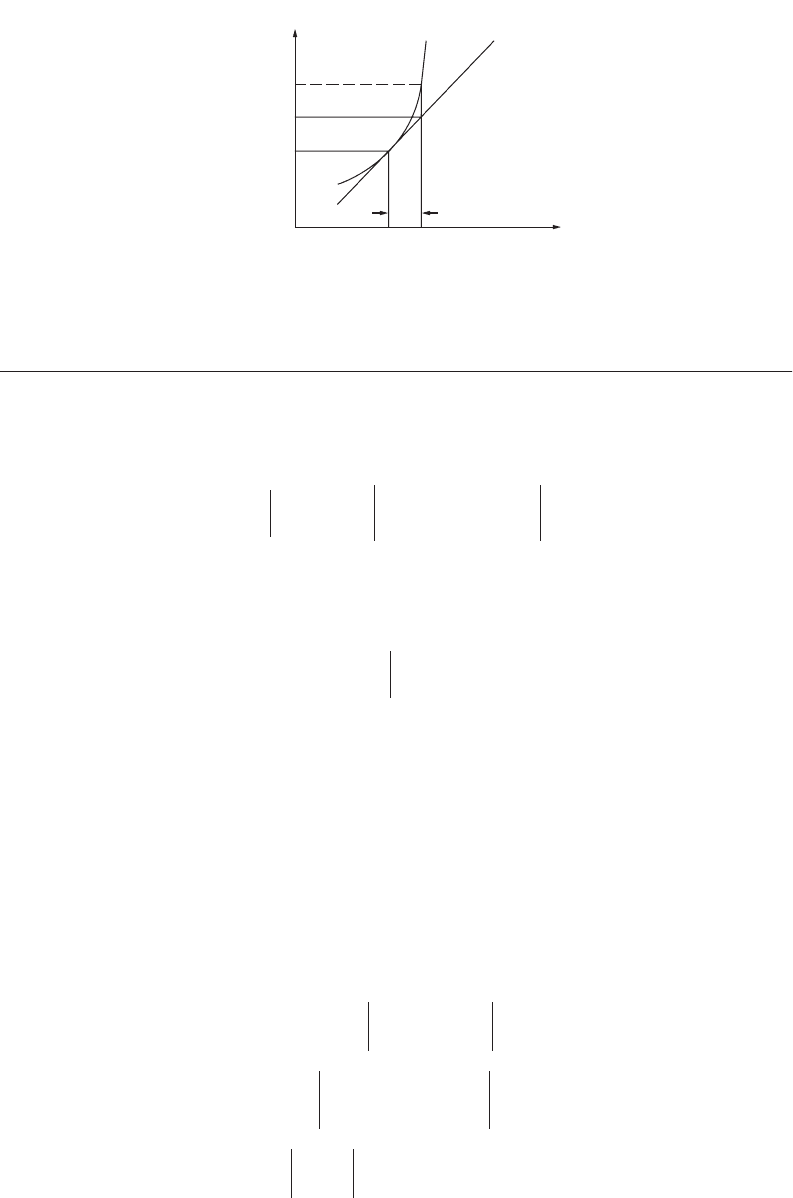
The technique of linearization is demonstrated in Fig. 53.4. The curve represents the original nonlinear

function f(x), whereas the straight line represents the linearized form, Eq. (53.122).

That line is tangent to the curve at the given point a, (x

0

, y

0

). When Dx is given (or evaluated), the

value of the function would be approximated by point b, whose ordinate is (y

0

+ jDx), and the exact value

from the nonlinear function is point c, with ordinate f (x

0

+ Dx). The error arising from using the linear

form is the line segment bc.

One Function of Two Variables

(53.123)

FIGURE 53.4 Linearization.

y

x

y

=

f

(

x

)

y

=

y

0

+

j

∆

x

(

y

0

+

j

∆

x

)

f

(

x

0

+ ∆

x

)

y

0

x

0

c

b

a

∆

x

yfx

0

()

df

dx

------

x

0

Dx

1

2!

----

d

2

y

dx

2

--------

x

0

Dx()

2

L

1

n!

-----

d

n

y

dx

n

--------

x

0

Dx()

n

L++ ++ +=

yfx

0

()

dy

dx

------

x

0

+ªDxy

0

jDx+ª

yfx

1

x

2

,()=

fx

1

0

x

2

0

,()

∂

y

∂

x

1

--------

x

1

0

x

2

0

,

Dx

1

∂

y

∂

x

2

--------

x

1

0

x

2

0

,

Dx

2

++=

1

2!

----

∂

2

y

∂

x

1

2

--------

x

1

0

x

2

0

,

Dx

1

()

2

1

2!

----

∂

2

y

∂

x

2

--------

x

1

0

x

2

0

,

Dx

2

()

2

++

∂

y

∂

x

1

--------

x

1

0

x

2

0

,

∂

y

∂

x

2

--------

x

1

0

x

2

0

,

Dx

1

()Dx

2

()L++

General Mathematical and Physical Concepts 53-31

For the linearized form, Eq. (53.123) is truncated to

(53.124)

where

Equation (53.124) can be rewritten in matrix form as

or

(53.125)

where

is the Jacobian of y with respect to x.

Two Functions of One Variable

(53.126)

or

with

Two Functions of Two Variables Each

(53.127a)

or

(53.127b)

or

(53.127c)

yy

0

j

1

Dx

1

j

2

Dx

2

++=

y

0

fx

1

0

x

2

0

,() j

1

∂

y

∂

x

1

--------

x

1

0

x

2

0

,

j

2

∂

y

∂

x

2

--------

x

1

0

x

2

0

,

===

yy

0

j

1

j

2

[]

Dx

1

D x

2

+=

yy

0

J

yx

Dx+=

J

yx

∂

y

∂

x

------

∂

y

∂

x

1

--------

∂

y

∂

x

2

--------

==

y

1

f

1

x() y

1

0

j

1

Dx+ª=

y

2

f

2

x() y

2

0

j

2

Dx+ª=

yy

0

J

yx

Dx+=

y

1

0

f

1

x

0

()=

y

2

0

f

2

x

0

()=

J

yx

j

1

j

2

[]

T

dy

1

dx

-------

x

0

dy

2

dx

-------

x

0

T

==

y

1

f

1

x

1

x

2

,()y

1

0

j

11

Dx

1

j

12

Dx

2

++ª=

y

2

f

2

x

1

x

2

,()y

2

0

j

21

Dx

1

j

22

Dx

2

++ª=

y

1

y

2

y

1

0

y

2

0

j

11

j

12

j

21

j

22

Dx

1

Dx

2

+ª

yy

0

J

yx

Dx+=

Wai-Fah Chen.The Civil Engineering Handbook

Подождите немного. Документ загружается.