Wai-Fah Chen.The Civil Engineering Handbook

Подождите немного. Документ загружается.

53-32 The Civil Engineering Handbook, Second Edition

where

and

evaluated at .

General Case of m Functions of n Variables

(53.128a)

With the auxiliaries,

the linearized form of Eq. (53.128a) becomes

(53.128b)

which represents the general form, with y, y

being vectors, J an Jacobian matrix, and Dx

an vector. Equations (53.122), (53.125), and (53.127c) are special cases of Eq. (53.128b).

,()

∂

------

∂

--------

∂

--------

∂

--------

∂

--------

º x

,, ,()=

º x

,, ,()=

º x

,, ,()=

º, x

,,()

º, x

,,()

º, x

,,()

∂

------

∂

--------

∂

--------

∂

--------

∂

---------

∂

---------

∂

---------

evaluated at x

Dx+ª

m 1¥ mn¥

n 1¥

General Mathematical and Physical Concepts 53-33

Differentiation of a Determinant

The partial derivative of a determinant with respect to a scalar is composed of the sum of p

determinants, each having the elements of only one row or one column replaced by their derivatives.

Thus, given the determinant in which represents its p columns, then

(53.129)

An expression similar to Eq. (53.129) can be written in which rows instead of the columns of d are

partially differentiated.

Differentiation of a Quotient

The partial derivative of g = U/W with respect to a variable x is given by

(53.130)

Both U and W can be general functions, including determinants, of several variables.

53.8 Map Projections

Map projection is concerned with the theory and techniques of proper representation of the curved earth

surface on the plane of a map. When the map is of such large scale as to represent a very limited area,

the earth curvature is insigniﬁcant, and ﬁeld survey measurements can be directly represented on the

map. On the other hand, as the surface area of the earth gets larger, this curvature becomes signiﬁcant

and must be dealt with. The earth is an ellipsoid and is also sometimes approximated by a sphere; neither

of these surfaces can accurately be developed into a plane. Therefore, all map projection methods must

by necessity contain some distortion. Various methods are selected to ﬁt best the shape of the area to be

mapped and to minimize the effects of particular distortions.

Locations on the earth are represented by meridians of longitude, l, and parallels of latitude, f. On

the map these are represented by scaled linear distances X, Y, using the dimensions of the earth ellipsoid

and selected criteria which the speciﬁc map projection must satisfy. These are obtained from transfor-

mation equations taking the general functional form of

(53.131)

Although all modern map projections are performed by computer programs, several are based on

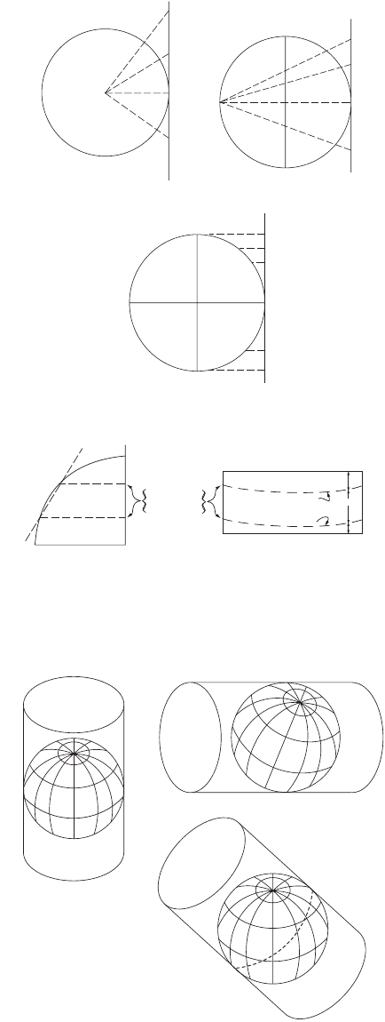
geometric projection of the earth onto one of three surfaces: a plane, a cylinder, or a cone. It is clear that

the cylinder and cone are chosen because they can be developed into a plane — that of the map. When

a plane is used, it is tangent to the earth’s surface at a point and the projection center is either the center

of the earth, as in the gnomonic projection shown in Fig. 53.5(a), or the point diametrically opposite to

the tangent point, as in the stereographic projection shown in Fig. 53.5(b). If the projection lines are

perpendicular to the plane, we have an orthographic projection, Fig. 53.5(c).

A cone is usually selected with its axis coincident with the earth’s polar axis. It may be tangent to the

earth at one small circle, called standard parallel, or intersect it in two standard parallels. When developed,

the scale will be true (i.e., without any distortion or error) at the standard parallels; see Fig. 53.6. Polyconic

projections use a series of frustums of cones, each from a separate cone.

Like a cone, a cylinder may be selected to be tangent to the earth or secant to it. It may be regular,

with its axis being the polar axis as in Fig. 53.7(a); transverse, with one tangent meridian as in Fig. 53.7(b);

secant, with two meridians of intersection; or oblique cylindrical, shown in Fig. 53.7(c).

pp¥

d D

L D

= D

i, 12Lp,=

∂

------

∂

----------

L D

∂

----------

L D

∂

---------

+++=

∂

------

-----

∂

-------

-----

∂

--------

–=

,()=

53-34 The Civil Engineering Handbook, Second Edition

FIGURE 53.5 (a) Gnomonic projection. (b) Stereographic projection. (c) Orthographic projection.

FIGURE 53.6 Lambert conformal conic projection. (Source: Davis, R. E., Foote, F. S., Anderson, J. M., and Mikhail,

E. M. 1981. Surveying: Theory and Practice, 6th ed., p. 570. McGraw-Hill, New York. With permission.)

FIGURE 53.7 (a) Vertical cylinder. (b) Transverse horizontal cylinder. (c) Oblique cylinder.

(a) (b)

(c)

′

Element of Cone

Standard

Parallels

Scale too large

Scale exact

Scale too small

(

)

Map of state

coordinate Zone

(

)

Section

(a)

(c)

(b)

General Mathematical and Physical Concepts 53-35

Equation (53.131) will produce a perfect map — without any distortions — if it satisﬁes all of the

following conditions:

1. All distances and areas have correct relative magnitudes.

2. All azimuths and angles are correctly represented on the map.

3. All great circles are shown on the map as straight lines.

4. Geodetic longitudes and latitudes are correctly shown on the map.

No one map projection can satisfy all these conditions. However, each class can satisfy some selected

conditions. The following are four classes:

1. Conformal or orthomorphic projection results in a map showing the correct angle between any

pair of short intersecting lines, thus making small areas appear in correct shape. As the scale varies

from point to point, the shapes of larger areas are incorrect.

2. An equal-area projection results in a map showing all areas in proper relative size, although these

areas may be much out of shape and the map may have other defects.

3. In an equidistant projection distances are correctly represented from one central point to other

points on the map.

4. In an azimuthal projection the map shows the correct direction or azimuth of any point relative

to one central point.

For conformal mapping, a new latitude, y, called the isometric latitude, is used in place of f, where

(53.132)

in which e

= (a

– b

)/a

, with a, b being the semimajor and semiminor axes of the earth ellipsoid,

respectively. Then, Eq. (53.131) is replaced by

(53.133)

In order for the mapping in Eq. (53.133) to be conformal, the following Cauchy–Riemann conditions

must be satisﬁed:

(53.134)

Two commonly used conformal projections are the Lambert conformal conic projection and the

transverse Mercator projection. A ﬁgure of the former is shown in Fig. 53.6, where the projection cone

intersects the ellipsoid in two standard parallels. It is very widely used in the U.S., particularly as a State

Plane Coordinate System for those states, or zones thereof, with greater east–west extent than north–south.

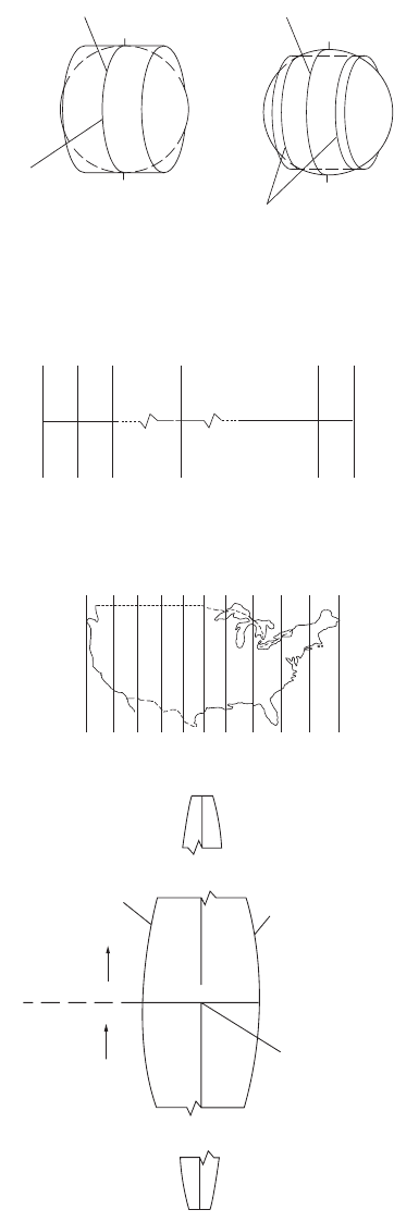
The transverse Mercator projection is shown in Fig. 53.8, where the cylinder is either tangent or secant

to the ellipsoid. When it is tangent, the scale at the central meridian is 1:1. But when it is not, the scale

at the central meridian is less than 1:1, as shown in Fig. 53.8. The central meridian is the origin of the

map X coordinate, while the origin of the map Y coordinate is the equator. This projection is used as a

State Plane Coordinate System for states with greater north–south extent.

An extensively used map projection system is the Universal Transverse Mercator, or UTM, schematically

shown in Fig. 53.9. It is in 6˚ wide zones, with the scale at each central meridian of a zone being 0.9996.

A false easting for each central meridian is 500,000 m. A transverse Mercator projection with 3˚ wide

zones is possible, where the scale at the central meridian is improved to 0.9999.

1 e

sin–

1 e

sin+

-----------------------

Ë¯

Êˆ

e 2§

---

---+

Ë¯

Êˆ

tan=

,()=

∂

∂l

-------

∂

∂y

-------

and

∂

∂y

-------

∂

∂l

------–==

53-36 The Civil Engineering Handbook, Second Edition

FIGURE 53.8 Tr ansverse Mercator projection. (a) Cylinder with one standard line. (b) Cylinder with two standard

lines.

FIGURE 53.9 (a) Universal Transverse Mercator zones. (b) UTM zones in the United States. (c) X and Y coordinates

of the origin of a UTM grid zone. (Source: U.S. Army Field Manual, Map Reading, FM 21-26.)

Central Meridian Central Meridian

Scale

1:1

Scale

1:1

(a) (b)

Zone

180°

168°

180°

0°

Equator

Zone number

10 11 12 13 14 15 16 17 18 19

(a)

(b) 126° 120°114°108°102°96° 90° 84° 78° 72° 66°

80°

south

10,000,000

m N

500,000

m E

central

meridian

m N

Meridian

3°

west

of central meridian

Meridian

3°

east

of central meridian

6°

zone

80°

north

Origin of zone

Equator

General Mathematical and Physical Concepts 53-37

53.9 Observational Data Adjustment

Mathematical Model for Adjustment

In surveying engineering, measurements are rarely used directly as the required information. They are

frequently used in subsequent operations to derive other quantities, often computationally, such as

directions, lengths, relative positions, areas, shapes, and volumes. The relationships applied in the com-

putational effort are the mathematical representations of the geometric and physical conditions of the

problem, which, together with the quality of the measurements, are called the mathematical model.

This mathematical model is composed of two parts: a functional model and a stochastic model. The

functional model is the part which describes the geometric or physical characteristics of the survey problem

and the resulting mathematical relationships. The stochastic model is the part of the mathematical model

that describes the statistical properties of all the elements involved in the functional model. It designates

which parts are the observables, which are constants, and which are unknown parameters to be estimated

in the adjustment. It also provides the information necessary to properly describe the quality of the

observations to be used in the adjustment.

As a simple example, consider the size and shape of a plane triangle. While the shape depends only

on angles, its size requires at least one side. Therefore, this model has three angular elements, the interior

angles, and three linear (or distance) elements, the triangle sides. Two angles and one side will be the

minimum number of measurements necessary to uniquely ﬁx the triangle. If more measurements than

these three are obtained, redundancy will exist, thus leading to inconsistency, which is resolved through

an adjustment technique. Once the number of measurements is decided upon, the required set of

independent condition equations can be written to express the functional model. The stochastic model

will denote those elements (of the total of six) which are observed, and the quality of the observations.

The a priori quality of an observed angle or distance is usually expressed by a standard deviation, s,

or its square, the variance, s

. Correlation between observations is represented by the covariance. Thus,

for two observables, or random variables, say and , the variances, and , and the covariance,

, are collected in a single square symmetric matrix called the variance-covariance matrix, or simply

the covariance matrix:

(53.135)

where the variances are along the main diagonal and the covariance off the diagonal. The concept of the

covariance matrix can be extended to the multidimensional case by considering n random variables

and writing

(53.136)

which is an square symmetric matrix.

Often in practice, the variances and covariances are not known in absolute terms but only to a scale

factor. The scale factor is given the symbol and is termed the reference variance, although other names,

such as “variance factor” and “variance associated with weight unity,” have also been used. The square

º x

,, ,

MOM

nn¥

53-38 The Civil Engineering Handbook, Second Edition

root , of , is called the “reference standard deviation” and was classically known as the “standard

error of unit weight.” The relative variances and covariances are called cofactors and are given by

(53.137)

Collecting the cofactors in a square symmetric matrix produces the cofactor matrix Q, with the obvious

relationship with the covariance matrix.

(53.138)

When Q is nonsingular, its inverse is called the weight matrix and designated by W; thus,

(53.139)

If is equal to 1, or, in other words, if the covariance matrix is known, the weight matrix becomes

its inverse.

Design/Preanalysis

Engineering design is more frequently known as preanalysis in surveying engineering. It refers to the task

of determining the observations to be made and their required accuracy so that the required accuracy

of the ﬁnal product is met. This is usually done by an iterative procedure, often using interactive graphics,

and applying the established mathematical model of the problem. The physical limitations of the project,

such as visibility and accessibility problems, are ﬁrst imposed on the design. Next, what is considered to

be an adequate set of measurements, with suitable accuracy estimates, is input in a design program to

estimate the required unknown parameters and their expected accuracy. The overall accuracy of the

estimated parameters is reﬂected by the posterior covariance matrix Â. (This is why preanalysis is

equivalent to covariance analysis used in the mathematical literature.) From Â, individual conﬁdence

measures, such as error ellipses and ellipsoids, are computed and compared to the design requirements.

If they are too large, additional observations or measurements of increased quality are attempted and

the process repeated. On the other hand, if they are too small (i.e., too good), reduced observations or

observations of decreased quality (using less expensive equipment/techniques) are attempted instead.

The procedure is iterated until an optimum design results.

Data Acquisition

The results of preanalysis provide the information required to set up the speciﬁcations for data acquisition,

particularly the quantities to be measured and their required accuracy. This leads to deciding on

equipment to be used and observational techniques to be applied. It is important that the selected

instruments be properly calibrated and in good working order, and that the procedures speciﬁed be

rigorously followed. Good ﬁeld practices must be followed to minimize blunders. In fact, all ﬁeld activities

are carefully planned and monitored so that the following operation, preprocessing of data, can be

effectively carried out to yield the most suitable data entering the adjustment.

Data Preprocessing

Preprocessing of survey data involves the elimination of blunders and the correction for all known

systematic errors. The resulting preprocessed measurements should have essentially nothing but random

errors before they are used in the adjustment. Any uncorrected systematic errors known to still exist in

the measurements must then be modeled mathematically and accounted for during the adjustment.

-----

and q

------==

-----

1–

General Mathematical and Physical Concepts 53-39

Because of the signiﬁcant cost of the ﬁeld operations, it is becoming more of a requirement to perform

preprocessing in the ﬁeld so as to minimize the cost of any remeasurement. Progressively more sophis-

ticated preprocessing programs are available for use with portable computers in conjunction with elec-

tronic data collectors.

There are several techniques for checking the observations which apply to the different types of

surveys, such as triangulation, trilateration, traverse, leveling, etc. These techniques depend on the shape

of the network and various minimum combinations of observations.

Data Adjustment

When redundant measurements exist, an adjustment of the observed data becomes necessary in order to

resolve the inconsistency between the observations and the model. As an illustration, consider the size

and shape of a plane triangle in which the three interior angles A, B, C and two sides a, b (opposite to

A and B, respectively) are measured. Suppose that we are interested in the length of the side c. We

obviously have more information than needed, since any one side, a or b, and any two angles sufﬁce to

solve the triangle and hence determine c. However, due to random measurement errors, every combina-

tion selected would be expected to lead to a slightly different value for c. A choice from all possible

combinations would be essentially arbitrary. More important is the fact that one should take advantage

of using all the available information in one operation, in which each measurement contributes relative

to its role in the mathematical model and commensurate with its quality (variance) relative to the quality

of all other measurements. One of the most commonly used techniques of adjustment of redundant

survey data is the method of least squares.

Least Squares Adjustment

Although least squares is an estimation procedure, it has been traditionally referred to in surveying as

an adjustment technique. This stems from the fact that after the adjustment the original observations are

replaced by a set of adjusted observations that are consistent with the model. Thus, after least squares

adjustment the ﬁve observations in the triangle example are replaced by a consistent set, in

that any minimum combination of these would yield the same triangle solution. Each adjusted observa-

tion is the sum of the original measurement and a residual, v, which is calculated in the adjustment.

The method of least squares is based on the observational residuals. If all the residuals in a given set

of n observations, 1 are denoted by the vector v, and the weight matrix associated with these observations

is W, the least squares criterion is given by

(53.140)

Note that f is a scalar, for which a minimum is obtained by equating to zero its partial derivatives with

respect to v. In Eq. (53.140) the weight matrix of the observations, W, may be full, implying that the

observations are correlated. If the observations are uncorrelated, W will be a diagonal matrix, and the

criterion simpliﬁes to

(53.141)

which says that the sum of the weighted squares of the residuals is a minimum. Another and simpler

case involves observations which are uncorrelated and of equal weight (precision), for which W = I, and

f becomes

(53.142)

,,,,,

Wv minimumÆ=

i 1=

minimumÆ++==

i 1=

ºv

minimumÆ++==

53-40 The Civil Engineering Handbook, Second Edition

The case covered by Eq. (53.142) is the oldest and may have accounted for the name “least squares,”

since it seeks the “least” sum of the squares of the residuals.

If we denote by n

the minimum number of independent variables needed to determine the selected

model uniquely, then the redundancy, r, is given by

(53.143)

As illustrations, consider the following examples.

1. The shape of a plane triangle is uniquely determined by a minimum of two interior angles, or

= 2. If three interior angles are measured, then, with n = 3, redundancy is r = 1.

2. The size and shape of a plane triangle require a minimum of three observations, at least one of

which is the length of one side, or n

= 3. If three interior angles and two side lengths are available,

then with n = 5 the redundancy is r = 2.

After the redundancy r is determined, the adjustment proceeds by writing equations that relate the

model variables in order to reﬂect the existing redundancy. Such equations will be referred to either as

condition equations or simply as conditions. The number of independent conditions, c, will be equal to r

if only observational variables and constants are involved. In many situations, however, additional

unknown variables, called parameters, are carried in the adjustment. In such a case, if the number of

unknown parameters is u, then a total of

c = r + u (53.144)

independent condition equations in terms of both the n observations and u parameters must be written.

In order for the parameter to be functionally independent, number, u, should not exceed the minimum

number of variables, n

, necessary to specify the model. Hence, the following relation must be satisﬁed:

0 £ u £ n

(53.145)

Similarly, for the formulated condition equations to be independent, their number, c, should not be

larger than the total number of observations n. Hence,

r £ c £ n (53.146)

Techniques of Least Squares

Although there is only one least squares criterion, there are several techniques by which least squares

may be applied. Regardless of which technique is applied, the results of an adjustment of a given set of

measurements associated with a speciﬁed model must be the same. The choice of a technique, therefore,

is mostly a matter of convenience and computational economy. The ﬁrst technique is called adjustment

of observations only. The condition equations take the form

(53.147)

For linear adjustment problems the vector f is given by

f = d = A1 (53.148)

in which d is a vector of numerical constants and 1 is the vector of given numerical values of the

measurements.

rnn

–=

rn,

n 1,

r 1,

General Mathematical and Physical Concepts 53-41

Let the cofactor matrix of the observations be denoted by Q( = W

–1

). Then

(53.149)

(53.150)

(53.151)

Error propagation:

(53.152)

(53.153)

(53.154)

The second technique is called adjustment of indirect observations. The condition equations are of

the general (nonlinear) form:

(53.155)

When linearized at approximations x

for the u = n

parameters x, they become

(53.156)

where D is a vector of unknown parameter corrections, is an n by u coefﬁcient matrix, and

f = – F(x

) –1. With W = Q

–1

( = S

–1

if s

= 1) as the weight matrix of the observations, then

(53.157)

(53.158)

(53.159)

(53.160)

Error propagation:

(53.161)

(53.162)

(53.163)

(53.164)

In the preceding technique, the largest number allowed for the parameters, u = n

, must be carried in the

adjustment so that each condition equation contains one and only one observation. In many applications,

kAQA

()

1–

f===

vQA

1v+=

AQ=

–=

--------------=

lvF++ x() 0=

v BDD

+ f=

∂F

∂x

------

WB=

Wf=

D N

1–

(iterate)+=

1–

Q Q

–=

--------------=