Alligood K., Sauer T., Yorke J.A. Chaos: An Introduction to Dynamical Systems

Подождите немного. Документ загружается.

C HAPTER T EN

Sta ble Ma n ifo ld s

and Crises

E INTRODUCED the subject of stable and unstable manifolds for saddles of

planar maps in Chapter 2. There we emphasized that Poincar

e used properties

of these sets to predict when systems would contain complicated dynamics. He

showed that if the stable and unstable manifolds crossed, there was behavior that

we now call chaos. For a saddle ﬁxed point in the plane, these “manifolds” are

curves that can be highly convoluted. In general, we cannot hope to describe the

manifolds with simple formulas, and we need to investigate properties that do

not depend on this knowledge. Recall that for an invertible map of the plane and

a ﬁxed point saddle p, the stable manifold of p is the set of initial points whose

forward orbits (under iteration by the map) converge to p, and the unstable

manifold of p is the set whose backward orbits (under iteration by the inverse of

the map) converge to p.

399

S TA B LE M ANIFOLDS AND C RISES

−π

−2

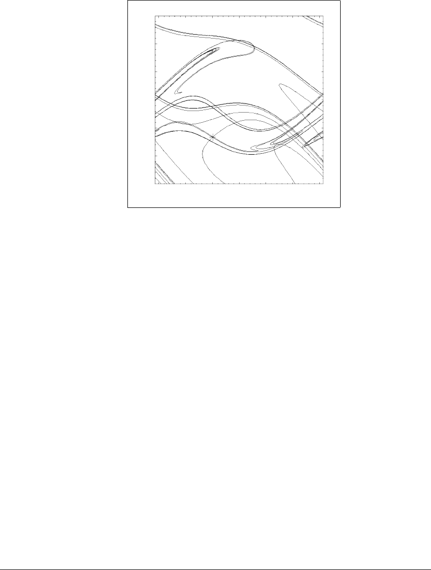
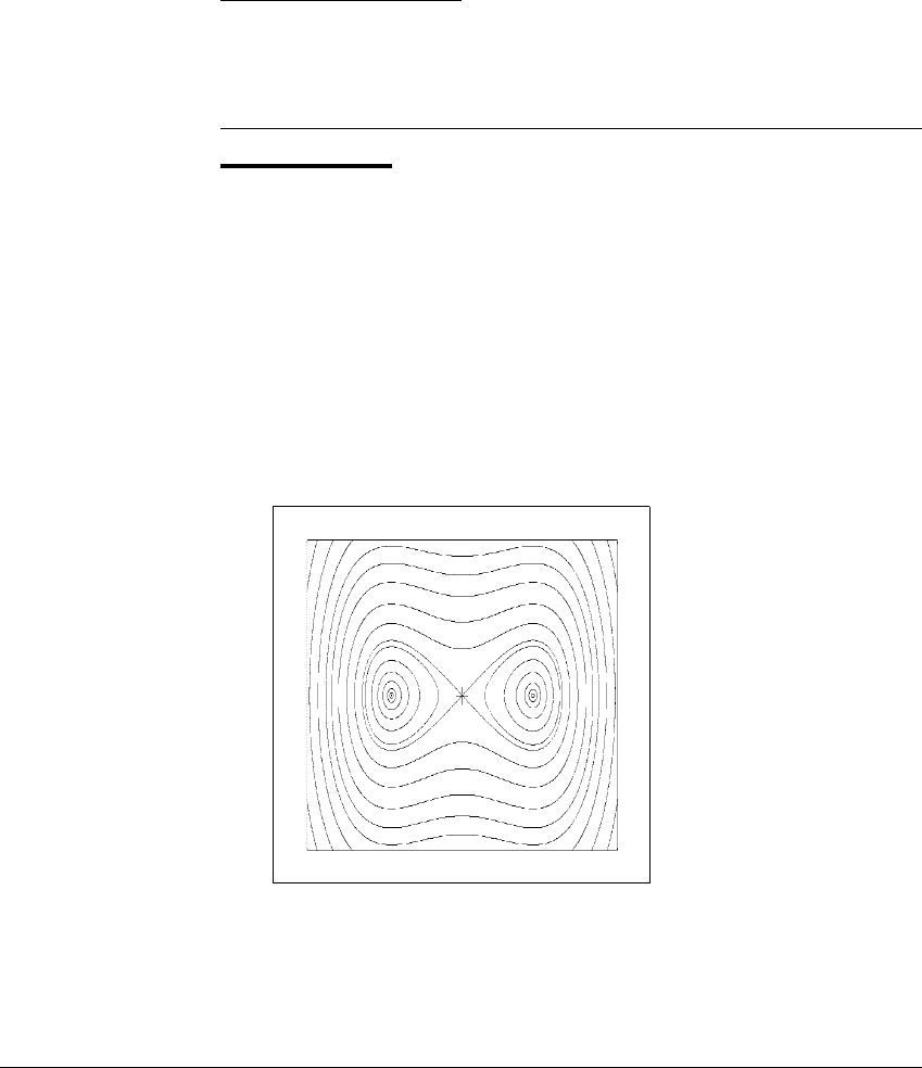
Figure 10.1 Stable and unstable manifolds for a ﬁxed point saddle the forced,

damped pendulum.

A cross marks a saddle ﬁxed point of the time-2

␲

map of the forced, damped

pendulum with equation of motion

x ⫹ .2

x ⫹ sin x ⫽ 2.5cost. The stable manifold

emanates from the saddle in the direction of an eigenvector V

⬇ (1, 0.88), and

the unstable manifold emanates from the saddle in the direction of an eigenvector

⬇ (1, ⫺0.59). A ﬁnite segment of each of these manifolds was computed. Larger

segments would show more complex patterns.

Figure 10.1 shows numerically calculated stable and unstable manifolds of

a saddle ﬁxed point of the time-2

␲

map of a forced damped pendulum, whose

motion satisﬁes the differential equation

x ⫹ .2

x ⫹ sin x ⫽ 2.5cost. The saddle

ﬁxed point p ⬇ (⫺.99, ⫺.33) is marked with a cross. The eigenvalues of the

Jacobian evaluated at p are s ⬇ ⫺0.13 and u ⬇ ⫺2.26. The stable manifold

S(p)

emanates from p in the direction of an eigenvector V

⬇ (1, 0.88) associated

with s, and the unstable manifold

U(p) emanates from p in the direction of an

eigenvector V

⬇ (1, ⫺0.59) associated with u. Although these manifolds are

far too complicated to be described by a simple formula, they still retain the form

of a one-dimensional curve we observed of all the examples in Chapter 2. Don’t

forget that points on the left side of the ﬁgure (at x ⫽⫺

␲

) match up with points

on the right side (at x ⫽

␲

), so that the curves, as far as they are calculated, have

no endpoints. It has been conjectured that the stable manifold comes arbitrarily

close to every point in the cylinder [⫺

␲

] ⫻ ⺢. Of course, here we have plotted

only a ﬁnite segment of that manifold.

400

10.1 THE S TABL E M ANIFOLD T HEOREM

The stable and unstable manifolds shown here look deceptively like tra-

jectories of a differential equation, except for the striking difference that these

curves cross each other. (The stable manifold does not cross itself, and the unsta-

ble manifold does not cross itself.) We stress that there is no contradiction here:

although distinct solutions of an autonomous differential equation in the plane

cannot cross, the stable and unstable manifolds of a saddle ﬁxed point of a plane

map are made up of inﬁnitely many distinct, discrete orbits. Points in the inter-

section of stable and unstable manifolds are points whose forward orbits converge

to the saddle (since they are in the stable manifold) and whose backward orbits

converge to the saddle (since they are in the unstable manifold). As we shall see

in Section 10.2, when stable and unstable manifolds cross, chaos follows.

We begin this chapter with an important theorem which guarantees that

the stable and unstable manifolds of a planar saddle are one-dimensional curves.

10.1 THE STABLE MANIFOLD THEOREM

For a linear map of the plane, the stable and unstable manifolds of a saddle are

lines in the direction of the eigenvectors. For nonlinear maps, as we have seen,

the manifolds can be curved and highly tangled. Just as with nonlinear sinks and

sources, however, more can be said about the structure of stable and unstable

manifolds for a nonlinear saddle by looking at the derivative, the Jacobian matrix

evaluated at the ﬁxed point. If, for example, 0 is a ﬁxed-point saddle of a map

f, then the stable and unstable manifolds of 0 under f are approximated in a

neighborhood of 0 by the stable and unstable manifolds of 0 under L(x) ⫽ Ax,

where A ⫽ Df(0). The relationship between the stable manifold of 0 under f

and of the stable manifold under Df(0) is given by the Stable Manifold Theorem,

the main result of this chapter.

Suppose, for example, we look at the map

f(x, y) ⫽ (.5x ⫹ g(x, y), 3y ⫹ h(x, y)),

where all terms of the functions g and h are of order two or greater in x and y;

functions like x

⫹ y

or xy ⫹ y

. Then the eigenvalues of Df(0)are.5and3,and

0 is a ﬁxed point saddle. We will see that the initial piece of the stable manifold

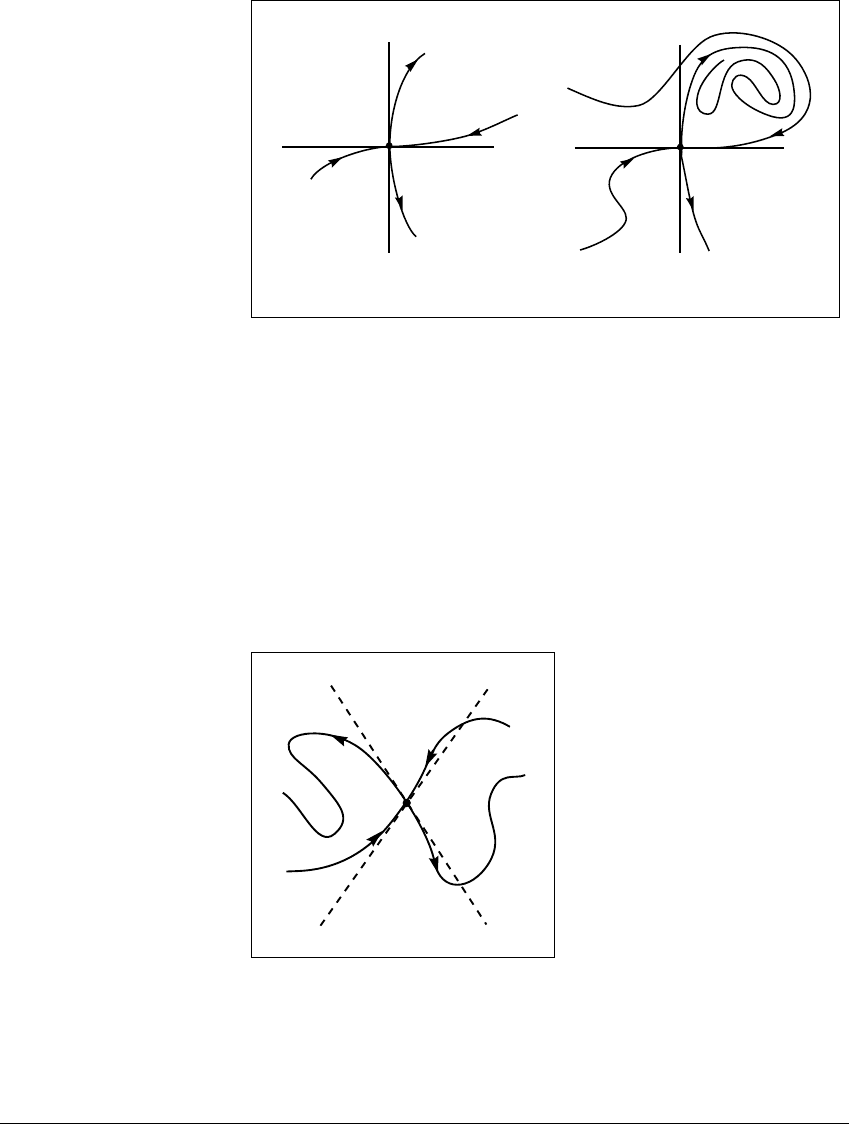
of 0, called the local stable manifold, emanates from 0 as the graph of a function

y ⫽

␾

(x). In addition, the x-axis is tangent to S at 0,thatis

␾



(0) ⫽ 0. See

Figure 10.2(a), which shows local stable and unstable manifolds. Globally, (that

is, beyond this initial piece), the stable manifold

S may wind around and not

be expressible as a function of x. It will, however, retain its one-dimensionality:

S is a smooth curve with no endpoints, corners, or crossing points. See Figure

401

S TA B LE M ANIFOLDS AND C RISES

y = h(x)

(a) (b)

Figure 10.2 Stable and unstable manifolds for a saddle in the plane.

(a) The local stable and unstable manifolds emanate from 0. (b) Globally, the stable

and unstable manifolds are one-dimensional manifolds.

10.2(b). We saw in Chapter 2 that such set is called a one-manifold. In the

case of a saddle in the plane, the stable manifold is the image of a one-to-one

differentiable function r, where r : ⺢ → ⺢

. The unstable manifold U(0)isalsoa

one-manifold that emanates from the origin in the direction of the y-axis. Figure

10.3 illustrates one-dimensional stable and unstable manifolds emanating from

the origin as described.

Figure 10.3 Illustration of the Stable Manifold Theorem.

The eigenvector V

is tangent to the stable manifold S at p, and the eigenvector

is tangent to the unstable manifold U. The manifolds are curves that can wind

through a region inﬁnitely many times. Here we show a ﬁnite segment of these

manifolds.

402

10.1 THE S TABL E M ANIFOLD T HEOREM

We state the theorem for a ﬁxed-point saddle in the plane and discuss

the higher-dimensional version in Sec. 10.5. The theorem says that the stable

and unstable manifolds are one-manifolds, in the topological sense, and that

they emanate from the ﬁxed point in the same direction as the corresponding

eigenvectors of the Jacobian. Figure 10.3 illustrates the theorem: The stable

manifold

S emanates from the saddle p in the direction of an eigenvector V

while the unstable manifold

U emanates in the direction of an eigenvector V

A corresponding version of the theorem holds for periodic points, in which

case each point in the periodic orbit has a stable and an unstable manifold. We

assume that maps are one-to-one with continuous inverses. Such maps are called

homeomorphisms. Smooth homeomorphisms (in which both the map and its

inverse are smooth) are called diffeomorphisms.

Theorem 10.1 (Stable Manifold Theorem.)Letf be a diffeomorphism of

⺢

. Assume that f has a ﬁ xed-point saddle p such that Df(p) has one eigenvalue s with

|s| ⬍ 1 and one eigenvalue u with |u| ⬎ 1.LetV

be an eigenvector corresponding to

s, and let V

be an eigenvector corresponding to u.

Then both the stable manifold

S of p and the unstable manifold U of p are one-

dimensional manifolds (curves) that contain p. Furthermore, the vector V

is tangent to

S at p,andV

is tangent to U at p.

Section 10.4 is devoted to a proof of the Stable Manifold Theorem. We end

this section with examples illustrating the theorem.

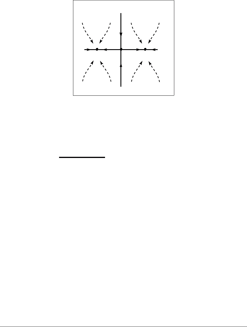
E XAMPLE 10.2

Let f(x, y) ⫽ ((4

␲

) arctan x, y 2). This map has two ﬁxed-point attrac-

tors, (⫺1, 0) and (1, 0), and a ﬁxed-point saddle (0, 0). The stable manifold of

(0, 0) is the y-axis. See Figure 10.4. The unstable manifold of (0, 0) is the set

兵(x, y):⫺1 ⬍ x ⬍ 1andy ⫽ 0其. The orbits of all points in the left half-plane

are attracted to (⫺1, 0), and those of points in the right half-plane are attracted

to (1, 0); i.e., these sets form the basins of attraction of the two attractors. (See

Chapter 3 for a more complete treatment of basins of attraction.) The stable

manifold of the saddle forms the boundary between the two basins. Focusing

here on the local behavior around the saddle ﬁxed-point (0, 0), we calculate the

eigenvalues of Df(0, 0) as s ⫽ 1 2andu ⫽ 4

␲

, with corresponding eigenvectors

⫽ (0, 1) and V

⫽ (1, 0), respectively. Thus the unstable and stable manifolds

emanate from (0, 0) in the directions of these vectors.

403

S TA B LE M ANIFOLDS AND C RISES

(1,0)(-1,0)

Figure 10.4 Action of the orbits for the map f(

x, y

) ⴝ ((4

␲

)arctan

x, y

 2)

The points (⫺1, 0) and (1, 0) are ﬁxed-point sinks, while the origin is a saddle.

The stable manifold of (0, 0) is the y-axis. The unstable manifold is the set 兵(x, 0) :

⫺1 ⬍ x ⬍ 1其.

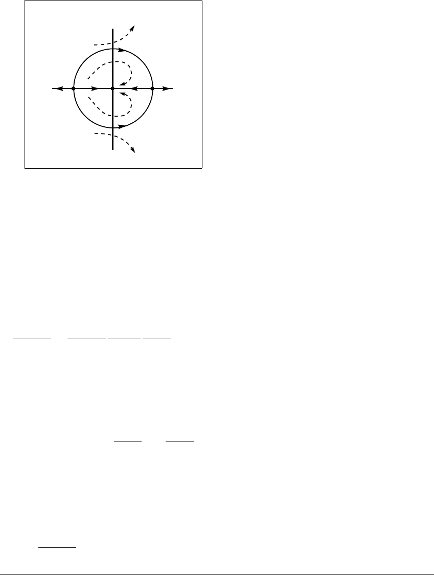
E XAMPLE 10.3

Let f(r,

␪

) ⫽ (r

␪

⫺ sin

␪

), where (r,

␪

) are polar coordinates in the plane.

There are three ﬁxed points: the origin and (r,

␪

) ⫽ (1, 0) and (1,

␲

). See Figure

10.5. The origin is a sink, attracting all points in the interior of the unit disk since

r → r

. There are two ways to compute the eigenvalues away from the origin.

One is to work in polar coordinates. Then

Df(r,

␪

) ⫽



2r 0

01⫺ cos

␪



for r ⬎ 0. The eigenvalues of each of the two ﬁxed points with r ⬎ 0 are easily

read from this diagonal matrix. The other way is to compute the eigenvalues in

rectangular coordinates. Since eigenvalues are independent of coordinates, the

results are the same. Checking the stability of the other two points in rectangular

coordinates allows us to review the chain rule for two variables.

The conversion between xy-coordinates and polar coordinates is x ⫽

r cos

␪

,y⫽ r sin

␪

.Themapf in terms of xy-coordinates is given by

F(x, y) ⫽





⫽



cos f

sin f



404

10.1 THE S TABL E M ANIFOLD T HEOREM

(-1,0)

(1,0)

Figure 10.5 Action of orbits for the map f(

r, ␪

) ⴝ (

, ␪

ⴚ sin

␪

)

Here (r,

␪

) are polar coordinates in the plane. In rectangular (x, y) coordinates, the

ﬁxed point (0, 0) is a sink; (⫺1, 0) is a source; and (1, 0) is a saddle. The stable

manifold of (1, 0) is the unit circle minus the ﬁxed point (⫺1, 0). The unstable

manifold of (1, 0) is the positive x-axis.

where f

(r,

␪

) ⫽ r

(r,

␪

) ⫽

␪

⫺ sin

␪

. The Jacobian of F with respect to rect-

angular coordinates is given by the chain rule:

⳵

)

⳵

(x, y)

⫽

⳵

)

⳵

)

⳵

)

⳵

(r,

␪

)

⳵

(r,

␪

)

⳵

(x, y)

⫽



cos f

⫺f

sin f

cos f



2r 0

01⫺ cos

␪



cos

␪

⫺r sin

␪

sin

␪

r cos

␪



⫺1

where we use the fact that the matrices of partial derivatives satisfy

⳵

(r,

␪

)

⳵

(x, y)

⫽



⳵

(x, y)

⳵

(r,

␪

)



⫺1

Now we can evaluate the rectangular coordinate Jacobian at the ﬁxed points

without actually converting the map to rectangular coordinates, which would be

quite a bit more complicated. At (r,

␪

) ⫽ (1, 0), or equivalently (x, y) ⫽ (1, 0),

we have

⳵

)

⳵

(x, y)

(1, 0) ⫽







⫺1

⫽





405

S TA B LE M ANIFOLDS AND C RISES

Thus D

f(1, 0) has eigenvalues s ⫽ 0andu ⫽ 2, with corresponding eigenvectors

⫽ (0, 1) and V

⫽ (1, 0). The stable manifold of this ﬁxed-point saddle is

given by the formula r ⫽ 1, ⫺

␲

⬍

␪

⬍

␲

. The unstable manifold is given by

r ⬎ 0,

␪

⫽ 0.

✎ E XERCISE T10.1

Repeat the computations of Example 10.3 for the other ﬁxed point (r,

␪

) ⫽

(1,

␲

), or (x, y ) ⫽ (⫺1, 0).

E XAMPLE 10.4

The phase plane of the double-well Dufﬁng equation

x ⫺ x ⫹ x

⫽ 0 (10.1)

is shown in Figure 10.6. This equation was introduced in Chapter 7. Here we in-

vestigate the stable and unstable manifolds under a time-T map. The equilibrium

(0, 0) of (10.1) is a saddle with eigenvectors V

⫽ (1, 1) and V

⫽ (1, ⫺1). These

vectors are tangent to a connecting arc as it emanates from the equilibrium and

then returns to it. Under the time-T map F

, all forward and backward iterates

Figure 10.6 Phase plane of the undamped Dufﬁng equation.

The phase plane of the two-well Dufﬁng equation

x ⫺ x ⫹ x

⫽ 0 is shown. The

equilibrium 0 (marked with a cross) is a ﬁxed point saddle of the time-T map. The

origin, together with the connecting arcs, form both the stable and the unstable

manifolds of 0 under the time-T map.

406

10.1 THE S TABL E M ANIFOLD T HEOREM

of initial conditions on a connecting arc remain on the arc. The origin is a ﬁxed

point saddle of F

, and the origin, together with the two connecting arcs, are

both the stable manifold and the unstable manifold of 0 under F

Although the previous examples illustrated the Stable Manifold Theorem,

we didn’t really use the theorem, since the stable and unstable manifolds could

be explicitly determined. (Recall that solution curves of the Dufﬁng phase plane

are level curves of the potential P(x) ⫽ x

 4 ⫺ x

 2.) We end this section with

enon map, an example in which the stable and unstable manifolds must be

approximated numerically. We outline the method used in all the numerically

calculated manifolds pictured in this book. The approximation begins by moving

in the direction of an eigenvector, as the theorem indicates.

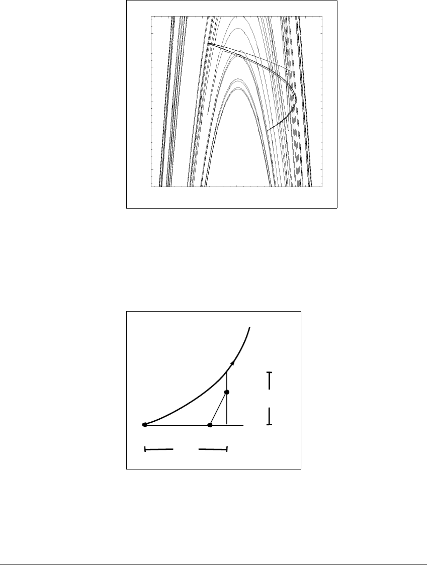
E XAMPLE 10.5

Let f(x, y) ⫽ (2.12 ⫺ x

⫺ .3y, x), one of the H

enon family of maps. Figure

10.7 shows stable and unstable manifolds of a ﬁxed-point saddle p ⬇ (.94,.94).

The eigenvalues of Df(p)ares ⬇ ⫺0.18 and u ⬇ ⫺1.71. The corresponding

eigenvectors are V

⬇ (1, ⫺5.71) and V

⬇ (1, ⫺.58). We describe a practical

method for approximating

U(p); S(p) can be approximated using the same algo-

rithm and f

⫺1

. First, ﬁnd (as we have done) an eigenvector V

associated with the

eigenvalue u. Choose a point a on the line through V

so that a and b ⫽ f(a)are

within 10

⫺6

of p. (If u happens to be negative, which is the case above, replace f

with f

here and throughout this discussion.)

If we assume that the unstable manifold is given locally as a quadratic

function of points on V

, then since |a ⫺ p| ⬍ 10

⫺6

, the distance of b ⫽ f(a)

from

U(p) is on the order of 10

⫺12

. See Figure 10.8. There might be extreme cases

where the distances 10

⫺6

and 10

⫺12

are too large, but such cases are very rare in

practice. Then apply f to the line segment ab ⫽ J. This involves choosing a grid

of points a ⫽ a

,...,a

⫽ b along the segment J. Let b

⫽ f(a

). The rule

used here is that the distance |b

⫺ b| should be less than 10

⫺3

. Otherwise, move

closer to a. Repeat this procedure when choosing each grid point. (Continue

with b

so that |b

⫺ b

| ⱕ 10

⫺3

, and so on.)

Using this method, calculate f, f

,...,f

of segment J. (Plot f(J) after it is

computed, then ignore the computation of f(J) when computing f

(J), etc.) At

some points, the computed value of f

(q) may be far from the actual value, due

to sensitive dependence. To avoid this problem, make sure that Df

(q)isnottoo

large. Plot only points q where each of the four entries in Df

(q)islessthan10

This will ensure that the error in f

(q), the distance to U(p), is on the order

of at most 10

⫺4

, assuming that f can be computed with an error of much less

407

S TA B LE M ANIFOLDS AND C RISES

2.5

−

2.5

−

2.5 2.5

Figure 10.7 Stable and unstable manifolds for a ﬁxed point saddle of the

enon map f(

x, y

) ⴝ (2

12 ⴚ

ⴚ

y, x

)

The ﬁxed point is marked with a cross. The unstable manifold is S-shaped; the stable

manifold is primarily vertical.

f(a)

-6

-12

U(p)

Figure 10.8 Calculating an unstable manifold.

Select a point a along an eigenvector V

so that a and f(a) are within 10

⫺6

the saddle p. Assuming that the unstable manifold is given locally as a quadratic

function of points on V

, then the distance of f(a)fromU(p) is on the order of

at most 10

⫺12

. Figure 10.7 and Color Plates 24–25 were created using the method

described in this section.

408