Baker K.R. Optimization Modeling with Spreadsheets

Подождите немного. Документ загружается.

SUMPRODUCT formula that we saw throughout Chapter 2. Box 3.1 summarizes the

prominent features of special networks.

One interesting feature of special network models is that an optimal solution

always consists of an integer-valued set of decision variables whenever the constraint

parameters are integer valued. Recall that the linearity assumption in linear program-

ming allows for divisibility in the values of decision variables. As a result, some or all

of the decision variables in an optimal solution may be fractional, and this sometimes

makes the result difﬁcult to implement or interpret. However, no such problem arises

with special networks; they will always lead to integer-valued solutions as long as the

constraint parameters are integers themselves.

Finally, the models of transportation, assignment, and transshipment problems

introduced thus far have featured LT constraints for capacities and GT constraints

for requirements, along with balance equations in the case of a transshipment

model. In the case of the assignment model, its special structure allowed us to use

equality constraints from the outset. However, as we shall discover next, it is possible

to formulate any of these problems as linear programs built exclusively on balance

equations. Although this approach may not seem as intuitive, it does link the ﬂow dia-

gram and the spreadsheet model more closely, as suggested at the beginning of the

chapter.

3.5. BUILDING NETWORK MODELS WITH

BALANCE EQUATIONS

The transportation model is a special kind of network. As we can readily see in the

diagram of Figure 3.1, the nodes can be partitioned into a set of supply locations

and a set of demand locations. This partitioning allows us to build a From/To structure

suited to the row-and-column format of the spreadsheet. However, we sometimes

encounter other network structures that do not lend themselves quite as easily to

an array layout for decision variables. For these networks, it may be desirable to for-

mulate the model using the standard linear programming format, with decision

variables in a single row and with a SUMPRODUCT function in each of the con-

straints. In what follows, we provide a glimpse of how to approach network models

in such a manner. The distinguishing feature of this approach is the use of balance

equations, relying heavily on the information in a ﬂow diagram. To illustrate how

this approach works, we return to examples we have already covered. As suggested

earlier, the balance equation approach is not the most intuitive way to handle transpor-

tation, assignment, and transshipment problems, but it will be useful background when

we analyze other network models. By revisiting the transportation, assignment, and

transshipment examples (Examples 3.1 –3.3) we can explore a new approach while

drawing on familiar problems.

The arcs of a network represent possible ﬂow paths, and the quantities ﬂowing

along each arc correspond to decision variables in the model. For diagramming pur-

poses, we also represent supply capacities and demand requirements as entering and

leaving arcs, respectively, just as in Figure 3.1 or 3.5. Now we take one additional

Chapter 3 Linear Programming: Network Models

step: we make sure that—for the entire network—the total supply quantity matches

the total demand quantity. This feature allows us to write a balance equation for

each node in the network.

Balanced totals for supply and demand occur in the assignment example of

Figure 3.5. Since the problem comes to us with that feature, we can move from the

diagram directly to the balance equations. For node A, the balance equation takes

the following form

ðFlow OutÞðFlow InÞ¼0

ðA1 þ A2 þ A3 þ A4 þ A5 þ A6Þ1 ¼ 0

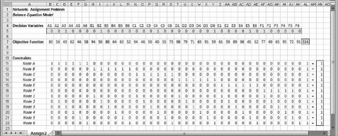
Similarly, there are 11 other balance equations. The full spreadsheet model, with 36

variables and 12 constraints, is shown in Figure 3.9. The optimal solution produced

by Solver achieves the minimum cost of $314 million, which we recognize from

Figure 3.6. The set of assignments matches the optimal solution in the earlier formu-

lation as well.

It is not hard to imagine a problem in which total supply and demand are unequal.

In fact, our transportation example in Figure 3.1 is just such a case. In this example,

total supply is 40,000, while total demand is 39,000. Thus, we might wonder

how to deal with problems that come to us with unbalanced totals for supply and

demand. Here is how we proceed. We alter the diagram by adding a “dummy” ware-

house to capture excess capacity. In our example, the requirement at this ﬁctitious

warehouse is 1000, bringing demand and capacity into balance. We then add arcs link-

ing each of the plants to the dummy warehouse, and we assign zero costs to these arcs.

We can think of shipments to the dummy warehouse as shipments to Nowhere.

In other words, ﬂows into the dummy warehouse are virtual ﬂows that do not actually

occur, whereas ﬂows into the ﬁrst four warehouses correspond to physical ﬂows.

The virtual ﬂows correspond to unused capacity, which justiﬁes using a cost of

zero on these arcs. The complete diagram is shown in Figure 3.10. We see that the

original diagram has been augmented so that there are now three capacities and ﬁve

Figure 3.9. Standard linear programming format for Example 3.2.

3.5. Building Network Models with Balance Equations 87

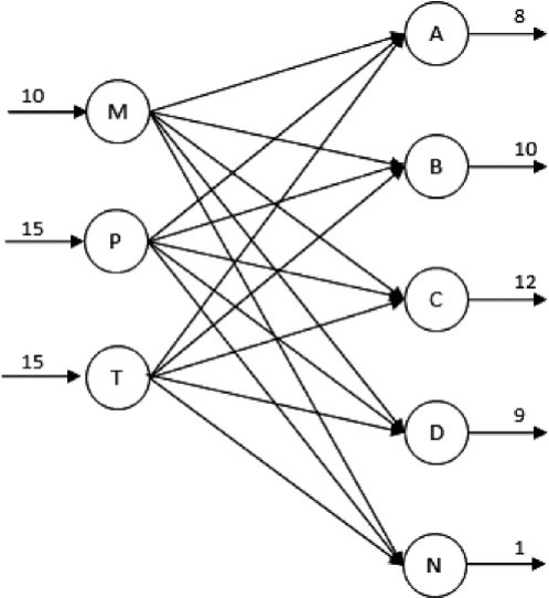
requirements, giving rise to eight nodes; and there are 15 routes, corresponding to

15 arcs. However, the net effect has been to recast the original network into an equiv-

alent one containing equal supply and demand quantities. This means that all of the

supply available at the plants must ultimately ﬁnd its way through the network to

the warehouses. As a result, there must be a balance equation for every node.

The next step is to translate the diagram into a linear programming model. We

again set aside one variable for each arc; thus, we reserve 15 columns for decision vari-

ables. There are also eight constraints, one corresponding to each node. The essential

requirement for any node in the model is a balance equation, that is, an EQ constraint

ensuring that total ﬂow into the node matches total ﬂow out of the node, or

(Flow Out)  (Flow In) ¼ 0

For example, at the Minneapolis node, the ﬂow in corresponds to the capacity of

10,000, while the ﬂows out correspond to the arcs (decision variables) MA, MB,

MC, MD, and MN. The balance equation becomes

MA þ MB þ MC þ MD þ MN  10,000 ¼ 0

or, in standard form, with variables on the left-hand side and constants on the right,

MA þ MB þ MC þ MD þ MN ¼ 10,000:

Figure 3.10. Flow diagram for the augmented version of Example 3.1.

88 Chapter 3 Linear Programming: Network Models

For the other two plants, we obtain

PA þ PB þ PC þ PD þ PN ¼ 15,000

TA þ TB þ TC þ TD þ TN ¼ 15,000

For the Atlanta node, the ﬂow in corresponds to the arcs MA, PA, and TA, while

the ﬂow out corresponds to the requirement of 8000. The balance equation becomes

8000  MA  PA  TA ¼ 0

which we choose to write as

MA  PA  TA ¼8000

For the other destination nodes, we obtain

MB  PB  TB ¼10,000

MC  PC  TC ¼12,000

MD  PD  TD ¼9000

MN  PN  TN ¼1000

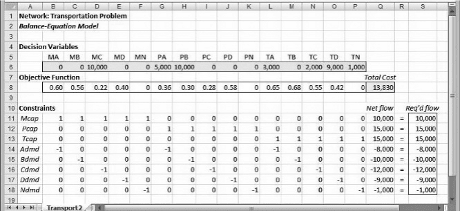
Figure 3.11 shows the complete spreadsheet model, in which all constraints are EQ

constraints, and the objective function is unchanged from before. Moreover, we can

distinguish ﬂows into the network as positive right-hand sides (in the ﬁrst three con-

straints) from ﬂows out of the network, which are negative right-hand sides (in the last

ﬁve constraints). The model speciﬁcation is as follows.

Objective: Q8 (minimize)

Variables: B6:P6

Constraints: Q11:Q18 ¼ S11:S18

Figure 3.11. Spreadsheet model for the augmented version of Example 3.1.

3.5. Building Network Models with Balance Equations 89

When we solve this optimization problem in the usual way, we obtain the same

minimum cost we saw previously, $13,830, as shown in Figure 3.11. In this case,

the decision variables also match those of Figure 3.2. The optimal solution also

contains the decision variable TN ¼ 1000, which we interpret as excess capacity of

1000 units at Tucson.

To summarize, we have followed a procedure for translating a network problem

into a linear program. This procedure requires a ﬂow diagram, possibly including

a dummy node to capture unused capacity. Once we construct such a diagram, we

can build the model by following these simple steps.

†

Deﬁne a variable for each arc.

†

Deﬁne a constraint for each node.

†

Express the balance equation for each node.

In addition, a sign convention for right-hand side constants can provide improved

clarity. Under this convention, a balance equation has a positive right-hand side to

signal ﬂow into the network and a negative right-hand side to signal ﬂow out of the

network.

For distribution problems of this sort, the From/To structure of the situation

lends itself most readily to the special network layout shown in Figure 3.2, and that

would be the modeling approach of choice. The approach suggested here is more

general and would be valuable in situations that are more complicated than transpor-

tation, assignment, or transshipment problems. We examine some examples in the

next section. Before we proceed, however, here is a perspective on the balance

equation model.

The special network models all adhere to the conservation law and the use of

balance equations, although it may be necessary to add a dummy node to make

sure that all supply capacity is consumed. In the models we built at the outset, the

addition of a dummy node and corresponding dummy arcs would have seemed

unwieldy or unnecessary. Fortunately, we were able to avoid that step and proceed

directly to a convenient formulation that contains inequalities rather than equations.

In effect, we were dropping the dummy nodes and arcs from the network. By ignoring

those virtual ﬂows, we could change the balance equation for each supply node to a LT

inequality. Similarly, we could also change the balance equation for each demand

node to a GT inequality, incorporating the additional ﬂexibility suggested in

Chapter 2. These simpliﬁcation steps left us with the network model we saw in

Figure 3.2, but with our new perspective, we can interpret it as an adaptation of the

balance equation model.

Special purpose solvers have been developed for use on large-scale network

problems in industry and academia. Typically, these solvers rely on balance equations

and therefore require that formulations contain equality constraints. However,

RSP does not presently have the facility to draw on these kinds of solvers. The

use of balance equations with Solver may help avoid formulation errors, but

it cannot exploit the algorithmic efﬁciencies that specialized network software

packages offer.

Chapter 3 Linear Programming: Network Models

3.6. GENERAL NETWORK MODELS WITH YIELDS

In network diagrams for the transportation, assignment, and transshipment models,

arcs carry ﬂow from one node to another. Moreover, on every arc, the ﬂow into the

destination node is implicitly required to exactly match the ﬂow sent out from

the source node. However, we can relax that kind of conservation requirement

and extend network models to cases in which ﬂows are subject to yield factors. The

yield factors may shrink the amount ﬂowing on an arc, in which cases we speak of

a yield loss. Alternatively, yield factors may enhance the amount ﬂowing, in which

case we speak of a yield gain. The next two subsections provide examples.

3.6.1. Models with Yield Losses

Yield loss occurs in manufacturing processes where materials are shaped and trimmed

to ﬁt a target design, thus creating material waste. In other settings, quality inspections

screen out defective parts. Process yields of these types reduce the amount of material

in the main product. Similarly, yield loss may occur in distribution processes,

especially with perishable goods. Fluids may partially evaporate during a delivery

trip, or vegetables may spoil. The net effect of perishability, as with process yields,

is simply a reduction in the amount of a ﬂow that reaches its destination.

EXAMPLE 3.4

The Goodwin Manufacturing Company Revisited

The Goodwin Manufacturing Company (of Example 3.1) ﬁnds that its product is subject

to evaporation in the tanker trucks used for distribution purposes. The average amount of evap-

oration depends the distance traveled and the average temperature. The following table shows

the corresponding yield loss as it has been observed to occur on each of its shipping routes.

(To) warehouse

(From) plant Atlanta Boston Chicago Denver

Minneapolis 0.24 0.19 0.07 0.11

Pittsburgh 0.10 0.05 0.04 0.15

Tucson 0.26 0.41 0.32 0.27

In this scenario, the yield factor tells us what proportion of the material sent along

an arc will reach its destination. For the purposes of decision making, we can still

measure the amounts sent out along each arc, but we have to adjust those ﬁgures to

determine how much demand is actually met at each destination. In addition, we

cannot know in advance how much material in the aggregate we will ship from the

three plants. We know that, after yield losses, we must ship more than the total

demand quantity (still 39,000), but we can’t tell how much more because we don’t

yet know which shipping routes we’ll use. Therefore, if we think of our model

3.6. General Network Models with Yields 91

containing a demand node for Nowhere, we must now treat the demand at that node as

a variable.

For the purposes of illustration, we assume that each plant has a standard capacity

of 16,000 units. Our supply constraints resemble those of the balance-equation model

of the previous section.

MA þ MB þ MC þ MD þ MN ¼ 10,000

PA þ PB þ PC þ PD þ PN ¼ 15,000

TA þ TB þ TC þ TD þ TN ¼ 15,000

For the Atlanta node, the ﬂow in corresponds to the net amounts on arcs MA, PA, and

TA, while the ﬂow out corresponds to the requirement of 8000. The balance equation

becomes

8000  0:76MA  0:90PA  0:74TA ¼ 0

which we choose to write as

0:76MA  0:90PA  0:74TA ¼8000

For the other destination nodes, we obtain

0:81MB  0:95PB  0:31TB ¼10,000



0:93MC  0:96PC  0:68TC ¼12,000

0:89MD  0:85PD  0:73TD ¼9000

MN  PN  TN  NX ¼ 0

In this last constraint, NX measures the total quantity unshipped and does not appear in

the objective function. The objective function is the same as the one we used initially.

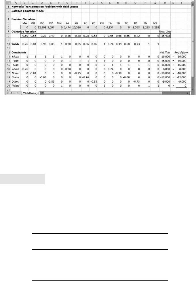
Figure 3.12 shows the complete spreadsheet model, in which all constraints are

EQ constraints, as in the previous section. In particular, the coefﬁcients in rows

16–20 are yield factors, and these values are taken from the parameters in row 10.

The model speciﬁcation is as follows.

Objective: R8 (minimize)

Variables: B6:Q6

Constraints: R13:R20 ¼ T13:T20

When we solve this optimization problem in the usual way, we obtain the mini-

mum cost of $15,498, as shown in Figure 3.12. To achieve this cost, the shipments out

of Minneapolis and Pittsburgh exhaust capacity, whereas some excess capacity

remains at Tucson. (The solution reﬂects this pattern because variables MN and PN

are zero, but TN is positive.) From the model, we can determine that the total quantity

shipped is 44,707, which provides the 39,000 units of demand after accounting

for yields.

With yields present in the model, the structure is not as simple as the transpor-

tation model, but we can exploit the conservation law to help us develop valid

constraints from balance equations.

Chapter 3 Linear Programming: Network Models

3.6.2. Models with Yield Gains

We look next at ﬂows that expand. Although there are chemicals that exhibit this prop-

erty, a more familiar application involves money. As money ﬂows through different

locations in time, it usually expands. This expansion results from drawing interest

or other kinds of investment returns. Consider the familiar problem of investing for

college expenses.

EXAMPLE 3.5

Planning for College

Two parents want to provide for their daughter’s college education with some money they

have recently inherited. They would like to set aside part of the inheritance in an account that

would cover the needs of their daughter’s college education, which begins four years from

now. They estimate that ﬁrst-year college expenses will come to $24,000 and increase $2000

per year during each of the remaining three years of college. The following investments are

available.

Investment Available Matures

Return at

maturity

A Every year 1 year 6%

B 1, 3, 5, 7 2 years 14%

C 1, 4 3 years 18%

D 1 7 years 65%

The parents would like to determine an investment plan that provides the necessary funds to

cover college expenses with the smallest initial investment. B

Figure 3.12. Spreadsheet model for Example 3.4.

3.6. General Network Models with Yields 93

Investment and funds-ﬂow problems of this sort lend themselves to network mod-

eling. In this type of problem, nodes represent points in time at which funds ﬂow could

occur. We can imagine tracking the balance in a bank account, with funds ﬂowing in

and out depending on our decisions. In Example 3.5, we include a node for now (time

zero), and nodes for the end of years 1 through 7. Tracking time for this purpose, the

end of year 3 and the start of year 4 are in effect the same point in time. To construct a

typical start-of-year node, we ﬁrst list the potential inﬂows and outﬂows that can occur.

Inﬂows

Initial investment

Appreciation of investment A from 1 year ago

Appreciation of investment B from 2 years ago

Appreciation of investment C from 3 years ago

Appreciation of investment D from 7 years ago

Outﬂows

Expense payment for the coming year

Investment in A for the coming year

Investment in B for the coming 2 years

Investment in C for the coming 3 years

Investment in D for the coming 7 years

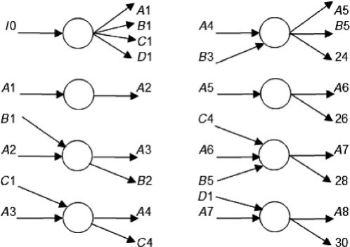
Not all of these inﬂows and outﬂows apply at every point in time, but if we sketch

the eight nodes and the ﬂows that do apply, we come up with a diagram such as the

Figure 3.13. Flow diagrams for Example 3.5.

94 Chapter 3 Linear Programming: Network Models

one shown as Figure 3.13. In this diagram, A1 represents the amount allocated to

Investment A at time zero, A2 represents the amount allocated to Investment A at

the start of year 2, and so on. The initial investment in the account is shown as I0,

and the expense payments are labeled with their numerical values. The diagram

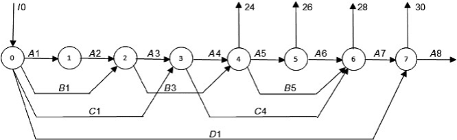
shows the different nodes as independent elements, which is all we really need; how-

ever, Figure 3.14 shows a tidier diagram in which the nodes are connected in a single

ﬂow network.

We do not need the variable B7 in the model. A 2-year investment starting in

year 7 would extend beyond the 8-year horizon, so this option is omitted. However,

the variable A8 does appear in the model. We can think of A8 as representing the

ﬁnal value in the account. Perhaps it is intuitive that, if we are trying to minimize

the initial investment, there is no reason to have money in the account in the end.

Still, to verify this intuition, we can include A8 in the model, anticipating that we

will ﬁnd A8 ¼ 0 in the optimal solution.

The next step is to convert the diagram into a linear programming model. For this

purpose, the ﬂows on the diagram become decision variables. Then, each node gives

rise to a balance equation, as listed below.

A1 þ B1 þ C1 þ D1  I0 ¼ 0 ðEnd of year 0Þ

A2  1:06A1 ¼ 0 ðEnd of year 1Þ

A3 þ B3  1:06A2  1:14B1 ¼ 0 ðEnd of year 2Þ

A4 þ C4  1:06A

3  1:18C1 ¼ 0 ðEnd of year 3Þ

A5 þ B5 þ 24,000  1:06A4  1:14B3 ¼ 0 ðEnd of year 4Þ

A6 þ 26,000  1:06A5 ¼ 0 ðEnd of year 5Þ

A7 þ 28,000  1:06A6  1:14B5  1: 18C4 ¼ 0 ðEnd of year 6Þ

A8 þ 30,000  1:06A7  1:65D1 ¼ 0 ðEnd of year 7Þ

Figure 3.15 shows these EQ constraints as part of the spreadsheet model. A

systematic pattern is formed by the coefﬁcients in the columns of the constraint

equations. Each column has two nonzero coefﬁcients: a positive coefﬁcient (of 1),

corresponding to the time the investment is made, and a negative coefﬁcient (reﬂecting

Figure 3.14. Uniﬁed ﬂow diagram for Example 3.5.

3.6. General Network Models with Yields 95