Baker K.R. Optimization Modeling with Spreadsheets
Подождите немного. Документ загружается.

Requirements per unit
STD DLX Hours available
Department 1 (hrs) 4 4 600
Department 2 (hrs) 3 2 400
Department 3 (hrs) 2 4 500
Profit per unit $50 $40
The Operations Manager at General Appliance would like to maximize profit contribution for
the month by choosing production quantities for the two models.
B
To formulate an optimization model for this scenario, let variables STD and DLX represent
the number of Standard and Deluxe models produced (and sold). If we represent the demand for
the Standard model by X, we can formulate the optimization problem for GAC as follows.
Maximize z ¼ 50 STD þ 30 DLX
subject to
4 STD þ 4 DLX 600
3 STD þ 2 DLX 400
2 STD þ 4 DLX 500
STD X
DLX 25
Thus, for any value of X, we can solve the optimization problem and determine the optimal pro-
duction quantities of STD and DLX.
In probability language, the possible demand scenarios are called states of nature
(or simply states), to indicate that the conditions are beyond our control. A probability
distribution lists the possible states and associates a probability with each state. (For
convenience, we’ll number th e states.) In our example, we might have some market
intelligence that leads us to adopt the following probability distribution.
State 1 2 3
Demand 80 104 160
Probability 0.2 0.5 0.3
Our optimization model takes three forms, depending on which state occurs. For state
1, the optimal output mix is 80 Standard models and 70 Deluxe models. For state 2, the
optimal output mix is 104 Standard models and 44 Deluxe models. Finally, for state 3,
the optimal output mix is 116.7 Standard models and 25 Deluxe models.
If we could learn the demand state in advance, we could determine the optimal
production quantity by solving the linear program with the appropriate demand
parameter. The crux of the problem, however, is that the production decision
must be determined before demand is known. Because we decide on production
396
Appendix 4 Stochastic Programming
before demand is resolved, there may be a di fference between the quantity pro-
duced and the quantity sold to retailers. (In the deterministic model, this difference
does not arise because feasible production quantities are sure to be sold.) The pro-
babilistic scenario forces us to consider what happens when production and sales
don’t match.
For the purposes of our example, suppose that GAC can sell its excess inventory
through a discount channel and earn a profit contribution of $15. Now, we must dis-
tinguish between the number of items produced and the number sold in each channel,
since those can differ when demand is stochastic. Thus, we introduce the variable SS1
to represent the number of Standard models sold to retailers in state 1 and SX1to
represent the number of excess Standard models (sold to the discounter) in state 1.
Then, our model requires two constraints.
SS1 80
STD SS1 SX1 ¼ 0
If production exceeds the demand of 80, then the first constraint limits retail sales to
demand, while the second constraint sets the excess equal to the difference between
production and retail sales. On the other hand, if demand exceeds production, then
the second constraint limits sales to production. (The excess quantity will then be
zero, because retail sales are more profitable than discount sales.) We do not need
to track the excess Deluxe models because all units of the Deluxe will be sold.
A similar set of constraint pairs is required for the other states.
State 2
SS2 104
STD SS2 SX2 ¼ 0
State 3
SS3 160
STD SS3 SX3 ¼ 0
Finally, we must account for the profits in a consistent manner, recognizing that
sales levels depend on which state occurs. For state 1, the objective function can be
expressed as follows.
Z1 ¼ 50SS1 þ 15SX1 þ 30DLX
Rearranging terms
50SS1 þ 15SX1 þ 30DLX Z1 ¼ 0
We next add this equality constraint to the model, as a means of defin ing Z1 internally.
For the other two states, we insert similar equalities.
50SS2 þ
15SX2 þ 30DLX Z2 ¼ 0
50SS3 þ 15SX3 þ 30DLX Z3 ¼ 0
A4.1. One-Stage Decisions with Uncertainty 397
Guided by the theory of decision making under uncertainty, our objective is to
maximize the expected value of profit. Having accounted separately for the profit in
each state, we can compute this expected value as a probability-weighted average,
using the following formula.
z ¼ 0:2Z1 þ 0:5Z2 þ 0:3Z3
This expression is linear, as are all of the additional constraints, so when we include
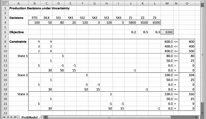
them in our model, we still have a linear programming problem. The full spreadsheet
model is displayed in Figure A4.1. The constraints have been organized into four sets.
The first set of (three) constraints carries over from the original model and includes the
production decisions, which must be determined before the uncertainty about demand
gets resolved. The next set of four constraints corresponds to state 1, th e following set
of four constraints corresponds to state 2 and the final set of four constraints corre-
sponds to state 3. The expected value of profit appears in the objective function.
Recall that the original deterministic model contained five constraints and
two variables. This new model contains 15 constraints and 11 variables, somewhat
more than in the original model. But these values depend directly on the number of
outcomes in our probability model. Had we represented demand with ten outcomes
instead of three, the model would contain 43 constraints and 25 variables.
Although we can reduce the problem size slightly by substituting for the
profit variables Z1, Z2, and Z3, the model is more transparent if the profit measure
is tracked separately for each state and then simply weighted in the objective function
to show the expected value calculation clearly. This is one of our design principles for
stochastic programming models.
Figure A4.1. Stochastic program for Example A4.1.
398 Appendix 4 Stochastic Programming

A second principle is to modularize the linear programming formulation by gath-
ering together the constraints that correspond to a given state. In our example, that
meant appending three constraint modules to the basic production-hours constraints.
Because the problem is stochastic, targets that might be met in one state may lead
to surplus or shortage in another state, so we must introduce additional variables to
track the consequences.
Finally, a third principle illustrated by our example spreadsheet is that the initial
decision variables reappear in each of the modules. In particular, the production
decision variables STD and DLX occur in the relevant demand constraints within
each of the three modules.
The optimal solution to the model, which achieves an expected profit of $6360, is
displayed in Figure A4.1. The optimal production mix is 100 Standard models and 50
Deluxe models, which corresponds to none of the output mixes produced by the model
for the individual scenarios.
The production of 100 Standard models and 50 Deluxe models represents a policy
that recognizes the risks due to uncertain demand. Under state 1, we have excess
Standard models and must accept the lower profit in the discount channel for some
of our output. On the other hand, under state 3, and to some extent under state 2,
we have a shortage of Standard models and must accept the lower profit from selling
Deluxe models instead. It would be feasible to produce a larger number of Deluxe
models, and those additional models would be certain to sell. But the profit available
from this strategy would not offset the expected loss es that would occur from pro-
ducing fewer Standard models because of limited resources. The need to balance
the risks arises because we have only one decision period. A two-period scenario is
discussed next.
A4.2. TWO-STAGE DECISIONS WITH UNCERTAINTY
In the one-stage model, a decision is made, and then the uncertain state is revealed.
At that point, all conditions are determined, and the economic consequences can be
computed. A more general structure is a two-stage model, which contains some oppor-
tunity to react to the uncertainty. The technical term for this structure is stochastic
programming with recourse. Again, we illustrate the principles with a modification
of Example A4.2.
EXAMPLE A4.2
General Appliance Company (continued)
Although monthly demand at GAC is uncertain, the uncertainty is resolved about half
way through the month. At that point, it is still possible to alter production plans slightly. In par-
ticular, GAC can reschedule during the last week of the month, enough to raise the available
hours in each department by 12 percent. Now, the Operations Manager faces a decision invol-
ving possible rescheduling as well as determining the output mix. B
A4.2. Two-Stage Decisions with Uncertainty
399
The addition to monthly capacity can be implemented after the demand state has been resolved.
Thus, 72 additional hours can be brought on line in department 1, 48 additional hours in depart-
ment 2, and 56 more in department 3. (The production capability might come, for example, from
an opportunity to schedule some unplanned overtime or simply by reassigning personnel.) How
does this new opportunity affect the decision?
As before, an initial production decision must be made before the demand state is
known. Should the level of demand be higher than expected, however, there is still an
opportunity to produce additional items, perhaps to fill the gap between the initial pro-
duction and the newly determined demand, or else to take advantage of the additional
capacity. In this second round of production decisions no uncertainty exists, and we
can proceed as if we were in a deterministic environment.
The analysis builds on the previous example. One new feature is an additional set
of production decisions corresponding to the second-stage. Thus, we define STD1 and
DLX1 as the Standa rd and Deluxe production quantities made with the additional
hours in the case of state 1. Similarly, STD2 and DLX2 represent the additional pro-
duction quantities for state 2, and STD3 and DLX3 represent the additional production
quantities for state 3.
Suppose that state 1 occurs after initial production decisions have been made. The
second-stage decision problem calls for choosing STD1 and DLX1 subject to three
resource constraints and the need to track any surplus that might occur. The module
of resource constraints takes the following form.
4 STD1 þ 4 DLX1 72
3 STD1 þ 2 DLX1 48
2 STD1 þ 4 DLX1 56
Next, with the second-stage production variables defined, we can modify the
definitional constraints of the one-stage example and add the following equations
for the state 1.
STD þ STD1 SX1 SS1 ¼ 0
SS1 80
DLX þ DLX1 25
Similar constraints apply to the other states.
State 2
STD þ STD2 SX2 SS2 ¼ 0
SS2 104
DLX þ
DLX2 25
State 3
STD þ STD3 SX3 SS3 ¼ 0
SS3 160
DLX þ DLX3 25
400
Appendix 4 Stochastic Programming
Finally, as in the previous example, we can capture the profits in auxiliary
variables.
50SS1 þ 15SX1 þ 30DLX þ 30DLX1 Z1 ¼ 0
50SS2 þ 15SX2 þ 30DLX þ 30DLX2 Z2 ¼ 0
50SS3 þ 15SX3 þ 30DLX þ 30DLX3 Z3 ¼ 0
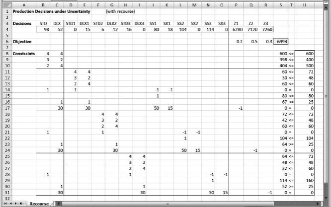
The entire model is shown in the spreadsheet of Figure A4.2. Here, again, the
model contains four modules, three of which correspond to the three demand states.
However, these are larger modules than in the one-stage example because of the
second production opportunity. For the two-stage model, we have 24 constraints
and 17 decision variables. Again, the model’s size depends on the number of states;
with ten states, our model would have 73 constraints and 45 decision variables.
Before we discuss the solution to the problem, we reiterate the three design
features shown in Figure A4.2.
†
A constraint module corresponds to each state.
†
The first-stage decisions appear in each of the modules corresponding to states.
†
Separate accounting is done for each of the objective function components that
correspond to states.
†
The objective function components are weighted by probabilities to construct
the overall expected value for the objective.
The solution displayed in Figure A4.2 has a complicated but logical pattern. The
initial production quantities are 98 Standard models and 52 Deluxe models. If state 1
occurs, the number of Standard models is already larger than demand, so additional
capacity will be devoted exclusively to 15 Deluxe models, bringing the total output
levels to 98 and 67. If state 2 occurs, the additional capacity will be used to bring
the number of Standard models up to retail demand and to add to the number of
Deluxe models, bringing the total output levels to 104 and 64. If state 3 occurs,
the additional capacity will be devoted exclusively to Standard models to the extent
available hours permit, bringing the totals to 114 and 52.
Thus, the initial production quantities leave several options open, and the optimal
plan takes one of three directions depending on the demand state. The expected profit
under the optimal plan is about $6994. By comparison , suppose we were to expand
the model in Figure A4.1 to reflect the full 112 percent capacity levels. The optimal
solution to that model (which has no recourse structure) achieves an expected profit
of only $6,952. Therefore, the ability to tailor our second-stage reactions to the sto-
chastic outcome allows us to achieve the greater profit level.
For another comparison, imagine that we could learn the demand state first and
then respond with a single production plan that had access to the incremental
12 percent capacity. For that situation, the expected profit (based on probabilities of
0.2, 0.5, and 0.3 for the three states, respectively) turns out to be $7103. It would
always be preferable to resolve uncertainty before making a production decision,
A4.2. Two-Stage Decisions with Uncertainty 401
but in this case, there is sufficient flexibility in the two-stage structure that the expected
profit is only about $109 lower for having to make the major decisions without know-
ing demand for sure. This low figure depends, of course, on the parameters of the
example, but it does suggest that the two-stage structure affords considerable flexi-
bility. Stochastic programming enables us to quantify this kind of flexibility.
A4.3. USING SOLVER
As described in Section A4.2, the optimization model for stochastic programming
with recourse can be viewed as an expanded linear program, with explicit treatment
of each random state. The expanded linear program can be developed and optimized
by running Solver. But keep in mind that our example contained essentially just five
constraints and two variables, only one of which was subject to uncertainty. Moreover,
that uncertainty was expressed in the form of a discrete probability distribution with
just three outcomes. For that small problem, the stochastic program was 24 by 17.
Stochastic programming models can become quite large, and constructing them can
be tedious and error-prone. We might wonder whether some of the modeling task
can be automated.
Risk Solver Platform has specialized capabilities for solving stochastic programs,
but to describe those capabilities, we must first examine its representation of probabil-
istic outcomes. RSP is an integrated software tool that uses probability distributions in
simulation models. A design feature in RSP is that only one simulation model can be
supported in a given workbook. Therefore, in building a stochastic programming
Figure A4.2. Stochastic program with recourse for Example A4.2.
402 Appendix 4 Stochastic Programming
model, or any simulation model, we should make sure that if our workbook contains
other worksheets, they do not contain probability distributions. (By contrast, RSP
supports one optimization model per worksheet.)
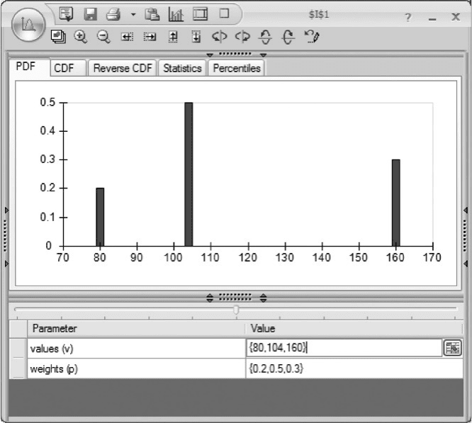
Suppose, for example, that we wish to construct a cell that behaves like demand
for Standard models in Exa mple A4.1. The relevant type of distribution in Solver is the
Discrete distribution, which we can access from the RSP ribbon via the Simulation
Model group of commands. Choose a cell to contain the demand model and select
Distributions
Q Custom Q Discrete. The Discrete distribution window offers the oppor-
tunity to specify values and weights, which are equivalent to outcomes and relative
probabilities. For our example of demand for Standard refrigerators, the values
would be {80, 104, 160} and the weights would be {0.2, 0.5, 0.3}. Entering these
values produces th e display shown in Figure A4.3.
By specifying the probability distribution for demand, we allow Solver to draw
samples from this distribution for the purposes of simulation. In general, a simulation
sample may not necessarily represent the relative probabilities in a distribution faith-
fully. In our example, if we draw 10 samples, we expect to obtain the value 80 about a
fifth of the time, which means twice. But in Monte Carlo sampling, we may draw the
Figure A4.3. Discrete distribution in risk solver platform.
A4.3. Using Solver 403
value 80 just once, or perhaps three times. Only in a large sample can we depend on
drawing the value 80 about 20 percent of the time. However, we can make the out-
comes conform much more closely to the given distribution by invoking Latin
Hypercube sampling. (This option can be selected by from the drop-down menu for
Options: select All Options and then select the Latin Hypercube radio button under
Sampling Method. In the same window, select All Trials as the Value to Display,
and set Trials per Simulation equal to 10.) Under Latin Hypercube sampling, a
sample of ten draws from the distribution will contain 80 twice, 104 five times, and
160 three times, conforming precisely to the frequencies in the given probability
model.
Because Solver has the capability of representing discrete probability models as
simulated outcomes, the stochastic program can be represented efficiently on a spread-
sheet. The recourse variables need only be represented once in the model. The spread-
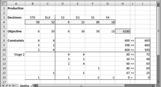
sheet model for Example A4.2 is shown in Figure A4.4.
In the spreadsheet model, the original variables are STD and DLX, as before. The
second stage decision variables are S2 and D2, representing the quantities produced
using the 12 percent resource capability at the second stage, and SS and SX,as
before, represent the number of Standard models sold to retailers and the number of
excess Standard m odels (sold to discounters). These last four decision variables are
designated Recourse variables in specifying the model elements in the task pane. In
addition, the demand di stribution is imbedded in cell J14.
The worksheet has only one explicit representation of the second stage, but Solver
can sample (10 times) for the value in cell J14, following the probability distribution.
1
Thus, Solver actually solves the problem two times with the demand outcome of 80 in
Figure A4.4. Solver model for the stochastic program of Example A4.2.
1
To obtain the optimal solution, we must set the Stochastic Transformation option on the Platform tab of
the task pane either to Deterministic Equivalent or to Automatic.
404 Appendix 4 Stochastic Programming
cell J14, five times with 104, and three times with 160. The corresponding optimal sol-
utions are stored and can be retrieved by clicking on the arrows in the Tools group on
the ribbon. When the number showing between the arrows is 1, the optimal solution
corresponding to the first simulation sample is displayed. When the number showing
is 2, the second sample is displayed, and so on. By clicking through the 10 outcomes,
we can verify that three sets of decisions appear, according to the demand outcome.
These sets of decisions, taken from row 4 of the worksheet, are summarized in the
table below.
Demand STD DLX S2 D2 SS SX
80 98 52 0 15 80 18
104 98 52 6 12 104 0
160 98 52 16 0 114 0
These results match those in Figure A4.2. However, the table layout makes it clearer
that the first-stage production quantities are 98 Standard models and 52 Deluxe
models, but the second-stage quantities depend on the demand outcome.
Finally, the expected-value objective function is not explicit in the worksheet for
Solver. However, to find the optimal value of the objective function, we can go to the
drop-down menu between the two arrows in the Tools group and select Sample Mean.
In place of the simulation trial number, the letter
m
appears. In addition the objective
function cell and the decision variable cells also display averages over the sample
outcomes. In the case of the objective function, the mean value corresponds to the
optimal value of the transformed model, in this case, $6994.
Stochastic programming can be a powerful form of analysis. It allows us to
address issues of uncertainty instead of making deterministic simp lifications. And
in the case of stochastic programming models with recourse, the solution helps us
tailor our responses to uncertain outcomes. However, there is a modeling cost for
this capability. Whereas a deterministic description allows us to meet targets exactly,
it is not possible to be as specific in a probabilistic setting. Instead, we may have to
invent variables to measure the surplus and shortage outcomes that occur when uncer-
tain factors are present. These new variables become part of a more complicated view
of the problem than we captured in the original, deterministic model. In addition, we
have to come up with a reasonable probability model for the uncertain elements of the
problem. In our example, we illustrated the use of a simple discrete distribution with
only three outcomes. In many cases, three outcomes might not be sufficient to provide
a meaningful description of the uncertainty. However, as we add outcomes to the
probability model, we expand the size of the model by requiring additional sets of
variables and constraints. Thus, accommodating even one source of uncertainty can
lead to an order of magnitude expansion in the size of the model. Modeling multiple
sources compounds this complexity. For these reasons, stochastic programming
models are still not widely used, but now that Solver can provide solutions, that situ-
ation may change.
A4.3. Using Solver 405